Linear classifiers: the perceptron and logistic regression

A linear classifier separates classes with a hyperplane. For two classes it computes a score \(f(\mathbf{x}) = \mathbf{w}^{\top}\mathbf{x} + b\) and predicts one class when the score is positive and the other when it is negative. The decision boundary \(\{\mathbf{x} : \mathbf{w}^{\top}\mathbf{x} + b = 0\}\) is a line in two dimensions, a plane in three and a hyperplane in general, and the weight vector w is perpendicular to it. Linear classifiers are fast to train, fast to apply, easy to inspect and surprisingly strong on high-dimensional data such as text, where a document is a vector with one entry per word. They are also the building block of neural networks, each of whose units is a linear function followed by a nonlinearity.

This lesson develops two classic linear classifiers. The perceptron, the first learning machine, illustrates online learning and comes with a beautiful convergence proof. Logistic regression, the workhorse of applied classification, outputs probabilities, has a convex training objective and a clear probabilistic interpretation, and extends naturally to many classes. Lesson 5 adds a third, the support vector machine, which chooses the separating hyperplane with the largest margin.

The perceptron

Frank Rosenblatt introduced the perceptron in 1958 at the Cornell Aeronautical Laboratory, and built it in hardware as the Mark I Perceptron, with an array of 400 photocells wired through motor-driven potentiometers. The learning rule is disarmingly simple. Use labels \(y \in \{-1, +1\}\), absorb the bias into w with a constant feature, and process training examples one at a time. If the current weights classify an example correctly, do nothing. If they misclassify it, that is if \(y_i \mathbf{w}^{\top}\mathbf{x}_i \le 0\), update

The update moves w toward \(\mathbf{x}_i\) for a positive example and away from it for a negative one, which increases \(y_i \mathbf{w}^{\top}\mathbf{x}_i\) by \(\lVert \mathbf{x}_i \rVert^2\), pushing the score on that example in the right direction. Repeat passes (epochs) over the data until a pass makes no mistakes.

The perceptron convergence theorem

Suppose the data are linearly separable with margin \(\gamma\): there is a unit vector \(\mathbf{w}^*\) with \(y_i \mathbf{w}^{*\top}\mathbf{x}_i \ge \gamma > 0\) for every example, and every input satisfies \(\lVert \mathbf{x}_i \rVert \le R\). Then the perceptron makes at most \((R/\gamma)^2\) mistakes, regardless of the order of the examples or the dimension of the space. The proof, due to Albert Novikoff in 1962, tracks two quantities after k mistakes, starting from \(\mathbf{w} = 0\).

First, alignment with the true direction grows at least linearly. Each mistake adds \(y_i \mathbf{x}_i\), and \(\mathbf{w}^{*\top}(y_i \mathbf{x}_i) \ge \gamma\), so after k mistakes \(\mathbf{w}^{*\top}\mathbf{w} \ge k\gamma\). Second, the length of w grows at most like a square root. On a mistake \(\lVert \mathbf{w} + y_i \mathbf{x}_i \rVert^2 = \lVert \mathbf{w} \rVert^2 + 2 y_i \mathbf{w}^{\top}\mathbf{x}_i + \lVert \mathbf{x}_i \rVert^2 \le \lVert \mathbf{w} \rVert^2 + R^2\), because the middle term is not positive on a mistake. So \(\lVert \mathbf{w} \rVert^2 \le kR^2\). Combining with the Cauchy–Schwarz inequality,

# The perceptron on linearly separable data, with the mistake bound (R / gamma)^2.
import numpy as np
rng = np.random.default_rng(367)
w_star = np.array([0.6, -0.8])                    # a unit-length separating direction
X = rng.uniform(-1, 1, size=(400, 2))
margin = X @ w_star
keep = np.abs(margin) > 0.1                       # remove points near the boundary: margin >= 0.1
X, y = X[keep], np.sign(margin[keep]).astype(int)  # labels in {-1, +1}

w = np.zeros(2); mistakes = 0
for epoch in range(1, 100):
    errors = 0
    for xi, yi in zip(X, y):
        if yi * (w @ xi) <= 0:                    # wrong side of (or on) the boundary
            w += yi * xi; mistakes += 1; errors += 1
    if errors == 0: break
R = np.max(np.linalg.norm(X, axis=1)); gamma = np.min(y * (X @ w_star))
print(f"{len(y)} points, converged after {epoch} passes and {mistakes} mistakes")
print(f"bound (R/gamma)^2 = ({R:.3f}/{gamma:.3f})^2 = {(R / gamma) ** 2:.0f}")
print(f"learned direction {np.round(w / np.linalg.norm(w), 3)} vs true {w_star}")

360 points, converged after 2 passes and 4 mistakes
bound (R/gamma)^2 = (1.353/0.102)^2 = 174
learned direction [ 0.67  -0.743] vs true [ 0.6 -0.8]

The bound is a worst case over all orderings; on typical data the perceptron makes far fewer mistakes. The theorem's significance is that the number of mistakes depends on the geometry of the data, the ratio of its radius to its margin, rather than on the number of features. That idea, that a large margin makes learning easy even in high dimensions, returns in lesson 5 with support vector machines.

The perceptron has serious limitations. If the data are not linearly separable, it never converges: the weights cycle forever. The averaged perceptron, which returns the average of the weight vectors over all steps, and the voted perceptron of Freund and Schapire fix this in practice and come with generalization guarantees. More fundamentally, a single linear unit cannot represent functions such as exclusive or, a point Marvin Minsky and Seymour Papert made forcefully in their 1969 book Perceptrons. Their analysis contributed to a decline of neural network research that lasted until multilayer networks trained by backpropagation revived it in the 1980s; lesson 12 shows how a hidden layer solves exclusive or.

Logistic regression

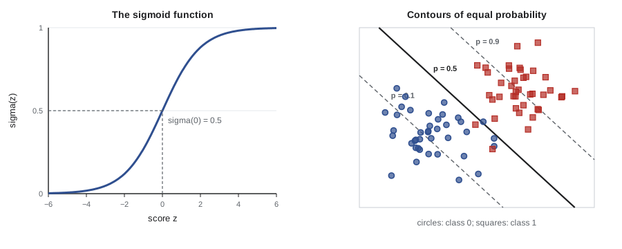
The perceptron outputs a hard decision. Many applications need a probability: a doctor wants the probability of disease, a lender the probability of default, and a spam filter benefits from knowing how confident it is. Logistic regression models the probability of the positive class (now with labels \(y \in \{0, 1\}\)) by passing the linear score through the logistic or sigmoid function:

The sigmoid squashes any real number into (0, 1), with \(\sigma(0) = 1/2\). Inverting it shows what the model assumes: the log odds, \(\log \frac{P(y=1 \mid \mathbf{x})}{P(y=0 \mid \mathbf{x})} = \mathbf{w}^{\top}\mathbf{x}\), are linear in the features. Each weight therefore has an interpretation: increasing feature j by one unit multiplies the odds of the positive class by \(e^{w_j}\). Predicting the positive class when the probability exceeds 1/2 gives a linear decision boundary at \(\mathbf{w}^{\top}\mathbf{x} = 0\); lesson 9 shows why other thresholds are often better.

Training by maximum likelihood

Given training data, the likelihood of the weights is \(\prod_i p_i^{y_i} (1 - p_i)^{1 - y_i}\) with \(p_i = \sigma(\mathbf{w}^{\top}\mathbf{x}_i)\). Its negative logarithm, averaged, is the cross-entropy or log loss:

The log loss punishes confident mistakes severely: predicting probability 0.01 for an example that turns out positive costs \(-\log 0.01 \approx 4.6\), while predicting 0.4 costs only 0.9. Unlike least squares, there is no closed-form minimizer. But J is convex, so any local minimum is global, and its gradient has a remarkably clean form. Using \(\sigma'(z) = \sigma(z)(1 - \sigma(z))\), the derivative of the loss for one example with respect to w simplifies to

which has the same form as the least squares gradient: prediction minus target, times the input. Gradient descent, Newton's method (which for logistic regression is called iteratively reweighted least squares) or quasi-Newton methods such as L-BFGS all work well; scikit-learn's default solver is L-BFGS. The program below implements plain gradient descent and checks the result against scikit-learn with the regularization effectively turned off.

# Logistic regression from scratch by gradient descent, checked against scikit-learn.
import numpy as np
from sklearn.linear_model import LogisticRegression
rng = np.random.default_rng(367)
# invented data: hours of study and practice problems done -> passed the exam (1) or not (0)
n = 300
hours = rng.uniform(0, 20, n); probs = rng.integers(0, 40, n)
logit = -6 + 0.35 * hours + 0.08 * probs
y = (rng.uniform(size=n) < 1 / (1 + np.exp(-logit))).astype(int)
X = np.column_stack([np.ones(n), hours, probs])

sigmoid = lambda z: 1 / (1 + np.exp(-z))
mu, sd = X[:, 1:].mean(axis=0), X[:, 1:].std(axis=0)
Z = np.column_stack([np.ones(n), (X[:, 1:] - mu) / sd])     # standardized copy for fast descent
v = np.zeros(3); lr = 0.5
for step in range(5000):
    p = sigmoid(Z @ v)
    v -= lr * Z.T @ (p - y) / n                    # gradient of the mean cross-entropy
w = np.r_[v[0] - np.sum(v[1:] * mu / sd), v[1:] / sd]       # weights on the original scale
p = sigmoid(X @ w)
loss = -np.mean(y * np.log(p) + (1 - y) * np.log(1 - p))
print("from scratch: w =", np.round(w, 3), f" mean log loss {loss:.4f}")
sk = LogisticRegression(C=1e6, max_iter=5000).fit(X[:, 1:], y)   # huge C = almost no penalty
print("scikit-learn: w =", np.round(np.r_[sk.intercept_, sk.coef_[0]], 3))
print(f"training accuracy {np.mean((p >= 0.5) == y):.3f}")
x_new = np.array([1, 12, 20])
print(f"P(pass | 12 hours, 20 problems) = {sigmoid(x_new @ w):.3f}")

from scratch: w = [-6.342  0.417  0.073]  mean log loss 0.3529
scikit-learn: w = [-6.342  0.417  0.073]
training accuracy 0.840
P(pass | 12 hours, 20 problems) = 0.530

The two sets of weights agree. They are close to, but not equal to, the values used to generate the data (−6, 0.35 and 0.08), the difference being sampling noise from only 300 examples. By the fitted model, each extra hour of study multiplies the odds of passing by about \(e^{0.42} \approx 1.5\). As in lesson 3, the descent runs on standardized features and the weights are converted back afterward; on the raw features, whose scales differ, plain gradient descent needs hundreds of thousands of steps to reach the same point. In practice one uses a library solver, but knowing that the gradient is just \(X^{\top}(\mathbf{p} - \mathbf{y})\) makes it easy to write the model into larger systems and to understand what the solver is doing.

Separable data and regularization

When the training data are linearly separable, the maximum likelihood weights do not exist: scaling w up makes every \(p_i\) closer to its label and the loss closer to zero, so the weights diverge to infinity. The fitted probabilities become 0 and 1 and the model is wildly overconfident. The same happens with many features relative to examples. The remedy is regularization, exactly as in lesson 3: add \(\lambda \lVert \mathbf{w} \rVert_2^2\) or \(\lambda \lVert \mathbf{w} \rVert_1\) to the loss. Scikit-learn's LogisticRegression applies an \(\ell_2\) penalty by default, parameterized by \(C = 1/\lambda\), so a small C means strong regularization; forgetting this default is a common source of puzzlement when comparing with other software.

Many classes: softmax regression

With K classes, multinomial logistic regression keeps a weight vector \(\mathbf{w}_k\) for each class and turns the K scores into probabilities with the softmax function:

The loss is again the cross-entropy, \(-\sum_i \log P(y_i \mid \mathbf{x}_i)\), and its gradient again has the form (predicted probabilities minus one-hot targets) times inputs. The decision regions are convex polygons bounded by the lines where two classes' scores are equal. When implementing softmax, subtract the largest score from all scores before exponentiating; the result is mathematically identical but avoids overflow. Softmax regression is exactly the output layer of a neural network classifier, which is why CMPUT-466 begins where this section ends.

# Multinomial (softmax) logistic regression on three invented classes.
import numpy as np
rng = np.random.default_rng(5)
means = np.array([[0, 0], [3, 1], [1, 3]])
X = np.vstack([rng.normal(c, 0.9, size=(100, 2)) for c in means])
y = np.repeat([0, 1, 2], 100)
Xb = np.column_stack([np.ones(len(X)), X]); Y = np.eye(3)[y]     # one-hot targets

def softmax(Z):
    Z = Z - Z.max(axis=1, keepdims=True)          # subtract the row maximum for numerical safety
    E = np.exp(Z); return E / E.sum(axis=1, keepdims=True)

W = np.zeros((3, 3)); lr = 0.1
for step in range(3000):
    P = softmax(Xb @ W)
    W -= lr * Xb.T @ (P - Y) / len(X)              # same form as the binary gradient
P = softmax(Xb @ W)
print(f"training accuracy {np.mean(P.argmax(axis=1) == y):.3f}")
print("class probabilities for the point (1.5, 1.5):", np.round(softmax(np.array([[1, 1.5, 1.5]]) @ W)[0], 3))

training accuracy 0.903
class probabilities for the point (1.5, 1.5): [0.151 0.398 0.45 ]

An alternative for K classes is to train K binary classifiers, each separating one class from the rest (one-versus-rest), or \(K(K-1)/2\) classifiers for every pair (one-versus-one), and combine their votes. These reductions let any binary method handle many classes; support vector machines often use them. Softmax regression is usually preferable for probabilistic linear models because it produces a single coherent set of probabilities.

Perceptron, logistic regression and the hinge loss

All linear classifiers share the same score \(f(\mathbf{x}) = \mathbf{w}^{\top}\mathbf{x}\); they differ in the loss they minimize, written as a function of the margin \(m = y f(\mathbf{x})\) with \(y \in \{-1, +1\}\). The 0-1 loss is 1 when \(m \le 0\). The perceptron effectively minimizes \(\max(0, -m)\), which ignores correct examples entirely. Logistic regression minimizes \(\log(1 + e^{-m})\), which keeps pushing for larger margins with diminishing force. The support vector machine of lesson 5 minimizes the hinge loss \(\max(0, 1 - m)\), which demands a margin of at least 1 and then stops caring. These surrogates are convex upper bounds (after scaling) on the 0-1 loss, which is what makes them tractable.

Interpreting and using linear classifiers

A linear classifier's weights are easy to inspect, which makes these models popular where decisions must be explained, such as credit scoring. Inspect them with care. A weight's size depends on its feature's scale, so compare standardized weights. Correlated features share credit unpredictably. And a weight describes association within the model, not cause: a credit model that gives weight to a postal code may be encoding neighborhood, income or ethnicity. Lending in Canada and the United States is subject to rules on explaining adverse decisions and on discrimination, and AI-460 discusses how to measure and mitigate unfair outcomes. For now, note that interpretability is a property of how a model is used and audited, not just of its functional form.

Worked examples