Ensembles: bagging, random forests and boosting

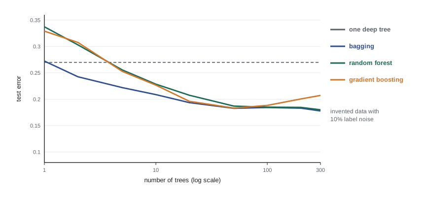
An ensemble combines the predictions of many models into one. The idea sounds like hedging, but it is one of the most powerful in machine learning: random forests and gradient-boosted trees are, for tabular data such as customer records, sensor logs and financial transactions, usually the most accurate off-the-shelf methods, and they regularly beat deep neural networks on such data. This lesson explains the two great families. Bagging and random forests average many high-variance models to cancel their errors. Boosting builds a sequence of weak models, each correcting its predecessors, to drive down bias. Both are most often applied to the decision trees of lesson 6.

Why averaging helps

Suppose we have B models whose errors on a given input are random variables with variance \(\sigma^2\) and pairwise correlation \(\rho\). The variance of their average is

As B grows, the second term vanishes, but the first does not: averaging removes the independent part of the errors and keeps the shared part. If the models were independent (\(\rho = 0\)), averaging B of them would divide the variance by B. If they were identical (\(\rho = 1\)), averaging would do nothing. Averaging leaves bias unchanged, because the average of the models has the same expected prediction as each one. So ensembles by averaging work best with models that have low bias, high variance and low correlation with each other. Unpruned decision trees fit that description perfectly: deep enough to have low bias, unstable enough to have high variance. The design problem is to make them as different from one another as possible.

Bagging

Leo Breiman's bagging (bootstrap aggregating, 1996) creates diversity by training each model on a different bootstrap sample: n examples drawn with replacement from the n training examples. Each bootstrap sample contains on average about 63.2 percent of the distinct examples, since the chance a given example is never drawn is \((1 - 1/n)^n \to e^{-1} \approx 0.368\). For regression the ensemble averages the predictions; for classification it takes a majority vote or averages predicted probabilities.

# Bagging from scratch: averaging trees grown on bootstrap samples reduces variance.
import numpy as np
from sklearn.tree import DecisionTreeRegressor
rng = np.random.default_rng(367)
f = lambda x: np.sin(3 * x) + 0.5 * x
def sample(n):
    x = rng.uniform(-2, 2, (n, 1)); return x, f(x[:, 0]) + rng.normal(0, 0.4, n)
Xtr, ytr = sample(150); Xte, yte = sample(3000)

def bagged(X, y, B):
    trees = []
    for b in range(B):
        idx = rng.integers(0, len(y), len(y))          # bootstrap: n draws with replacement
        trees.append(DecisionTreeRegressor(random_state=b).fit(X[idx], y[idx]))
    return lambda Xq: np.mean([t.predict(Xq) for t in trees], axis=0)

single = DecisionTreeRegressor(random_state=0).fit(Xtr, ytr)
print(f"one unpruned tree:    test MSE {np.mean((single.predict(Xte) - yte) ** 2):.3f}")
for B in (5, 25, 100):
    print(f"bagging, B = {B:3}:    test MSE {np.mean((bagged(Xtr, ytr, B)(Xte) - yte) ** 2):.3f}")
print("noise variance (the floor): 0.160")
print(f"fraction of distinct examples in a bootstrap sample of 150: {np.unique(rng.integers(0, 150, 150)).size / 150:.3f}")

one unpruned tree:    test MSE 0.329
bagging, B =   5:    test MSE 0.249
bagging, B =  25:    test MSE 0.237
bagging, B = 100:    test MSE 0.239
noise variance (the floor): 0.160
fraction of distinct examples in a bootstrap sample of 150: 0.680

A single unpruned tree has test error about twice the noise floor; bagging only 5 trees cuts the error by a quarter, 25 trees help a little more, and beyond that the error levels off, because the variance that remains is the part the trees share. Bagging rarely hurts: adding more trees does not cause overfitting in the way that adding depth does, because each new tree only refines an average. It helps little for stable, low-variance models such as linear regression, and it is most useful for exactly the models, like deep trees, that a statistician would call unreliable.

Bagging also offers a free validation set. Each example is left out of about 37 percent of the bootstrap samples. Predicting each example using only the trees that did not see it gives the out-of-bag (OOB) error, an estimate of test error almost as good as cross-validation and obtained at no extra cost.

Random forests

Trees grown on bootstrap samples of the same data are still strongly correlated: if one feature is a strong predictor, nearly every tree will split on it at the root, and the trees will look alike. Breiman's random forests (2001) add a second source of randomness: at each split, only a random subset of m of the d features is considered. A common default is \(m \approx \sqrt{d}\) for classification and \(m \approx d/3\) for regression. Forcing trees to use different features decorrelates them, lowering \(\rho\) in the variance formula, and the forest's accuracy improves even though each individual tree is somewhat worse.

Random forests have few hyperparameters and are forgiving about their values: the number of trees (more is better, with diminishing returns), m, and the minimum leaf size. They need no feature scaling, handle mixed feature types, give OOB error estimates and are trivially parallel. These qualities make a random forest an excellent first model to try on a new tabular problem, and a strong baseline against which to judge more elaborate methods.

Feature importance

Forests are less interpretable than a single tree, but they offer measures of how much each feature matters. Impurity-based importance (mean decrease in impurity) adds up the impurity reduction from every split on a feature, across all trees. It is cheap but biased toward features with many distinct values, which offer many candidate thresholds and so can reduce training impurity by chance. Permutation importance measures how much a model's accuracy on held-out data drops when one feature's values are randomly shuffled, breaking its relationship with the target. It is more reliable, applies to any model, and should be computed on validation or test data rather than training data.

# A random forest with out-of-bag error and two kinds of feature importance.
import numpy as np
from sklearn.ensemble import RandomForestClassifier
from sklearn.inspection import permutation_importance
rng = np.random.default_rng(367)
# invented data: will a shipment arrive late? Only the first three features matter.
n = 1500
names = ["distance", "storm", "holiday", "weight", "box_id"]
X = np.column_stack([rng.uniform(0, 2000, n), rng.integers(0, 2, n), rng.integers(0, 2, n),
                     rng.uniform(1, 30, n), rng.integers(0, 100_000, n)])
logit = -3 + 0.0015 * X[:, 0] + 1.6 * X[:, 1] + 1.0 * X[:, 2]
y = (rng.uniform(size=n) < 1 / (1 + np.exp(-logit))).astype(int)
Xtr, ytr, Xte, yte = X[:1000], y[:1000], X[1000:], y[1000:]

rf = RandomForestClassifier(n_estimators=300, oob_score=True, random_state=0).fit(Xtr, ytr)
print(f"out-of-bag accuracy {rf.oob_score_:.3f}   test accuracy {rf.score(Xte, yte):.3f}")
perm = permutation_importance(rf, Xte, yte, n_repeats=20, random_state=0)
print("feature    impurity importance   permutation importance (test set)")
for i in np.argsort(-perm.importances_mean):
    print(f"{names[i]:9}  {rf.feature_importances_[i]:19.3f}   {perm.importances_mean[i]:22.3f}")

out-of-bag accuracy 0.669   test accuracy 0.664
feature    impurity importance   permutation importance (test set)
distance                 0.353                    0.071
storm                    0.121                    0.054
holiday                  0.048                    0.014
box_id                   0.239                   -0.004
weight                   0.239                   -0.009

The meaningless box identifier, a number between 0 and 100,000, and the irrelevant weight, a continuous measurement, together receive almost half of the impurity importance, more than storm and holiday combined, because their many distinct values let trees split on them repeatedly to fit noise in the training data. Their permutation importances on test data are about zero (slightly negative, which is just noise), correctly revealing them as useless. Both measures agree that distance, storm and holiday matter. Neither measure says anything about causation, and both can mislead when features are strongly correlated, since shuffling one of a correlated pair leaves its partner to carry the information.

Boosting

Boosting answers a question posed by Michael Kearns and Leslie Valiant in 1988: can a weak learner, one that is only slightly better than random guessing, be turned into a strong learner with arbitrarily small error? Robert Schapire showed in 1990 that it can, and Yoav Freund and Schapire's AdaBoost (1995), which earned them the 2003 Gödel Prize, made the idea practical. Where bagging trains models independently and in parallel, boosting trains them in sequence, each one focusing on the examples its predecessors got wrong.

AdaBoost

AdaBoost keeps a weight on every training example, initially uniform. In round m it trains a weak learner \(h_m\), typically a decision stump, to minimize weighted error \(\varepsilon_m\). It gives the learner a vote \(\alpha_m = \frac{1}{2} \ln \frac{1 - \varepsilon_m}{\varepsilon_m}\), which is large when the error is small. Then it reweights the examples, multiplying each weight by \(e^{-\alpha_m y_i h_m(x_i)}\) and renormalizing, so that misclassified examples gain weight and correctly classified ones lose it. The final classifier is a weighted vote:

If every weak learner has weighted error at most \(1/2 - \gamma\), the training error of the vote falls exponentially, at most \(e^{-2\gamma^2 M}\) after M rounds. Later analysis by Friedman, Hastie and Tibshirani showed that AdaBoost is stagewise minimization of the exponential loss \(e^{-y F(x)}\), another convex surrogate for the 0-1 loss, which connected boosting to the rest of statistical learning.

# AdaBoost with decision stumps, written from scratch.
import numpy as np
rng = np.random.default_rng(4)
n = 400
X = rng.uniform(-1, 1, (n, 2))
y = np.where(X[:, 0] ** 2 + X[:, 1] ** 2 < 0.45, 1, -1)       # a circle: no single stump can fit it
Xte = rng.uniform(-1, 1, (4000, 2)); yte = np.where(Xte[:, 0] ** 2 + Xte[:, 1] ** 2 < 0.45, 1, -1)

def best_stump(X, y, w):
    best = (np.inf, None)
    for j in range(X.shape[1]):
        for t in np.unique(X[:, j]):
            for s in (1, -1):
                pred = np.where(X[:, j] < t, s, -s)
                err = w[pred != y].sum()
                if err < best[0]: best = (err, (j, t, s))
    return best

def stump_predict(X, j, t, s): return np.where(X[:, j] < t, s, -s)

w = np.full(n, 1 / n); F_tr = np.zeros(n); F_te = np.zeros(len(yte))
print("round  weighted error  alpha   train error  test error")
for m in range(1, 101):
    err, (j, t, s) = best_stump(X, y, w)
    alpha = 0.5 * np.log((1 - err) / err)
    h = stump_predict(X, j, t, s)
    w *= np.exp(-alpha * y * h); w /= w.sum()                 # up-weight the mistakes
    F_tr += alpha * h; F_te += alpha * stump_predict(Xte, j, t, s)
    if m in (1, 2, 5, 20, 50, 100):
        print(f"{m:5}  {err:14.3f}  {alpha:5.3f}  {np.mean(np.sign(F_tr) != y):11.3f}  {np.mean(np.sign(F_te) != yte):10.3f}")

round  weighted error  alpha   train error  test error
    1           0.343  0.326        0.343       0.355
    2           0.331  0.352        0.435       0.462
    5           0.383  0.238        0.152       0.202
   20           0.393  0.217        0.040       0.085
   50           0.404  0.194        0.010       0.045
  100           0.416  0.170        0.003       0.043

One stump can only cut the square with a single line, so its error is large. As rounds accumulate, the weighted vote of axis-aligned cuts builds an approximation to the circle, and both training and test error fall. Note that the weighted error of later stumps approaches one half: AdaBoost keeps concentrating weight on the hard examples near the boundary, where no single stump does much better than guessing. Remarkably, AdaBoost's test error often keeps falling after its training error reaches zero, which a margin-based analysis by Schapire, Freund, Bartlett and Lee explained: further rounds increase the margins of the training examples. AdaBoost is, however, sensitive to label noise, since it keeps increasing the weight of mislabeled examples it can never fit.

Gradient boosting

Jerome Friedman's gradient boosting (1999–2001) generalizes boosting to any differentiable loss. The model is an additive expansion \(F_M(\mathbf{x}) = F_0 + \nu \sum_{m=1}^{M} h_m(\mathbf{x})\). At each stage, compute the negative gradient of the loss with respect to the current predictions at each training point, called pseudo-residuals, fit a small regression tree to them, and add it, scaled by a learning rate \(\nu\):

For squared loss the pseudo-residuals are ordinary residuals \(y_i - F_{m-1}(\mathbf{x}_i)\), so each tree literally fits what the ensemble has not yet explained. For log loss they are \(y_i - p_i\), and the same machinery gives a boosted classifier. Gradient boosting is gradient descent in function space: each tree is a step in the direction that most reduces the loss.

# Gradient boosting for regression from scratch: each small tree fits the current residuals.
import numpy as np
from sklearn.tree import DecisionTreeRegressor
from sklearn.ensemble import GradientBoostingRegressor
rng = np.random.default_rng(367)
f = lambda x: np.sin(3 * x[:, 0]) + 0.5 * x[:, 1] ** 2
def sample(n):
    X = rng.uniform(-2, 2, (n, 2)); return X, f(X) + rng.normal(0, 0.3, n)
Xtr, ytr = sample(500); Xte, yte = sample(3000)

nu, M = 0.1, 300                                   # learning rate (shrinkage) and number of trees
F_tr = np.full(len(ytr), ytr.mean()); F_te = np.full(len(yte), ytr.mean())
for m in range(1, M + 1):
    resid = ytr - F_tr                             # negative gradient of squared loss
    tree = DecisionTreeRegressor(max_depth=3, random_state=m).fit(Xtr, resid)
    F_tr += nu * tree.predict(Xtr); F_te += nu * tree.predict(Xte)
    if m in (1, 10, 50, 100, 300):
        print(f"trees {m:3}: train MSE {np.mean((F_tr - ytr) ** 2):.3f}   test MSE {np.mean((F_te - yte) ** 2):.3f}")
sk = GradientBoostingRegressor(n_estimators=M, learning_rate=nu, max_depth=3, random_state=0).fit(Xtr, ytr)
print(f"scikit-learn, same settings: test MSE {np.mean((sk.predict(Xte) - yte) ** 2):.3f}  (noise floor 0.090)")

trees   1: train MSE 0.906   test MSE 0.889
trees  10: train MSE 0.390   test MSE 0.442
trees  50: train MSE 0.073   test MSE 0.126
trees 100: train MSE 0.049   test MSE 0.112
trees 300: train MSE 0.023   test MSE 0.119
scikit-learn, same settings: test MSE 0.119  (noise floor 0.090)

In the run above, test error is lowest at around 100 trees and has begun to creep up by 300, even though training error keeps falling. Unlike bagging, boosting can overfit if run too long, because each new tree fits more of the training residual, including noise. The defenses are shrinkage (a small learning rate such as 0.1 or 0.05, with more trees), shallow trees (depth 3 to 8), subsampling rows and columns for each tree (stochastic gradient boosting), and early stopping when validation error stops improving. The learning rate and the number of trees trade off against each other: halving \(\nu\) roughly doubles the trees needed but usually gives slightly better results.

Modern boosting libraries

Three open-source libraries dominate practice. XGBoost (Tianqi Chen and Carlos Guestrin, 2016) added second-order gradient information, explicit regularization of tree complexity, sparsity-aware split finding and careful systems engineering; it became famous through its record in data science competitions. LightGBM (Microsoft, 2017) grows trees leaf-wise and bins feature values into histograms for speed on large data. CatBoost (Yandex, 2017) handles categorical features with ordered target statistics that avoid a subtle form of leakage. Scikit-learn's HistGradientBoostingClassifier and HistGradientBoostingRegressor provide a fast histogram-based implementation in the standard library. All share Friedman's core algorithm; the differences matter for speed, memory and the handling of categorical and missing values more than for the underlying idea.

Stacking and other combinations

Ensembles need not be homogeneous. Stacking, introduced by David Wolpert in 1992, trains several different models (say a logistic regression, an SVM and a random forest) and then a second-level model that learns how to combine their predictions. To avoid leakage, the second-level model must be trained on out-of-fold predictions: predictions for each training example made by first-level models that did not see it during training, produced by the cross-validation procedure of lesson 9. Simple averaging of diverse strong models is a surprisingly hard baseline to beat, and the winning entries in many prediction competitions, including the Netflix Prize in 2009, have been large blends.

Worked examples