Support vector machines and kernels

Among all the hyperplanes that separate two classes, which one should a classifier choose? The perceptron stops at the first one it finds; logistic regression, unregularized, wanders off to infinity. Support vector machines (SVMs) give a principled answer: choose the hyperplane that maximizes the margin, the distance to the nearest training points. Combined with the kernel trick, which lets a linear method operate in an enormous or even infinite-dimensional feature space at modest cost, SVMs were the most successful general-purpose classifiers from the mid-1990s until the deep learning era, and they remain an excellent choice for small and medium-sized data sets with many features.

The ideas trace to Vladimir Vapnik and Alexey Chervonenkis's work on optimal separating hyperplanes in the 1960s; the modern soft-margin SVM with kernels was published by Corinna Cortes and Vapnik in 1995, building on Bernhard Boser, Isabelle Guyon and Vapnik's 1992 kernel paper. This lesson develops the maximum-margin idea, the soft margin and hinge loss, the dual problem and support vectors, kernels and Mercer's condition, and kernel ridge regression. The full optimization theory (Lagrangian duality and the KKT conditions) belongs to AI-310; here we use its results.

The geometric margin

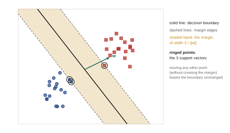
For a linear classifier \(f(\mathbf{x}) = \mathbf{w}^{\top}\mathbf{x} + b\) with labels \(y \in \{-1, +1\}\), the signed distance of a point from the hyperplane is \(f(\mathbf{x}) / \lVert \mathbf{w} \rVert\). The geometric margin of a correctly classified example is \(y_i f(\mathbf{x}_i) / \lVert \mathbf{w} \rVert\), and the margin of the classifier on a data set is the smallest such value. Because scaling w and b by the same constant does not change the hyperplane, we can fix the scale by requiring \(y_i f(\mathbf{x}_i) \ge 1\) for every example, with equality for the closest points. The margin is then \(1/\lVert \mathbf{w} \rVert\) on each side, and maximizing it is the same as minimizing \(\lVert \mathbf{w} \rVert^2\). The hard-margin SVM solves

This is a convex quadratic program with a unique solution. Why prefer the largest margin? Intuitively, a boundary far from every training point is robust: small perturbations of the inputs, or new points drawn near the old ones, stay on the correct side. Formally, margin-based generalization bounds show that the error of a large-margin classifier depends on \((R/\gamma)^2\), the same quantity as the perceptron mistake bound, rather than on the dimension of the space. That is why SVMs can work in feature spaces with far more dimensions than training examples.

The soft margin and the hinge loss

Real data are rarely separable, and even when they are, one mislabeled point can force a narrow margin. The soft-margin SVM allows violations through slack variables \(\xi_i \ge 0\):

A point with \(0 < \xi_i \le 1\) lies inside the margin but on the correct side; \(\xi_i > 1\) means it is misclassified. The constant C sets the price of violations. A large C insists on fitting the training data and gives a narrow margin (low bias, high variance); a small C tolerates violations for a wider margin (more bias, less variance). At the optimum each slack equals \(\max(0, 1 - y_i f(\mathbf{x}_i))\), so the problem can be rewritten without constraints as regularized hinge loss minimization:

This form shows that an SVM is a linear classifier with the hinge loss and an \(\ell_2\) penalty, exactly parallel to ridge regression and regularized logistic regression. It also suggests a simple training algorithm. The hinge loss is convex but not differentiable at margin 1, so we use a subgradient: \(-y_i \mathbf{x}_i\) when the margin is below 1 and 0 otherwise. Pegasos (Shalev-Shwartz, Singer and Srebro, 2007) runs stochastic subgradient descent with step size \(1/(\lambda t)\) and scales to millions of examples.

# A linear soft-margin SVM trained by Pegasos (stochastic subgradient descent on the hinge loss).
import numpy as np
from sklearn.svm import SVC
rng = np.random.default_rng(367)
n = 200
X = np.vstack([rng.normal([-1.5, -1.0], 0.8, (n // 2, 2)), rng.normal([1.5, 1.0], 0.8, (n // 2, 2))])
y = np.r_[-np.ones(n // 2), np.ones(n // 2)]
Xb = np.column_stack([X, np.ones(n)])            # bias as a third weight (Pegasos penalizes it slightly)

lam = 0.01; w = np.zeros(3)
for t in range(1, 50_001):
    i = rng.integers(n)
    eta = 1 / (lam * t)                           # the Pegasos step-size schedule
    if y[i] * (w @ Xb[i]) < 1:                    # inside the margin or misclassified
        w = (1 - eta * lam) * w + eta * y[i] * Xb[i]
    else:
        w = (1 - eta * lam) * w
obj = lam / 2 * w[:2] @ w[:2] + np.mean(np.maximum(0, 1 - y * (Xb @ w)))
print("Pegasos:      w =", np.round(w, 3), f" objective {obj:.4f}")
svc = SVC(kernel="linear", C=1 / (lam * n)).fit(X, y)    # the same problem in scikit-learn's form
print("scikit-learn: w =", np.round(np.r_[svc.coef_[0], svc.intercept_], 3))
m = 2 / np.linalg.norm(svc.coef_[0])
print(f"margin width 2/||w|| = {m:.3f}; support vectors: {len(svc.support_)} of {n}")
print(f"training accuracy {np.mean(svc.predict(X) == y):.3f}")

Pegasos:      w = [ 1.269  1.174 -0.252]  objective 0.0434
scikit-learn: w = [ 1.297  1.184 -0.272]
margin width 2/||w|| = 1.139; support vectors: 12 of 200
training accuracy 0.990

Pegasos lands close to the exact solution computed by scikit-learn's SVC (which wraps the LIBSVM library). The small differences come from the stochastic updates and from Pegasos treating the bias as an ordinary, slightly penalized weight. Note how few of the 200 examples are support vectors: the solution depends only on the points on or inside the margin.

The dual problem and support vectors

Lagrangian duality converts the soft-margin problem into an equivalent problem over one multiplier \(\alpha_i\) per training example:

with the weights recovered as \(\mathbf{w} = \sum_i \alpha_i y_i \mathbf{x}_i\). Two facts about the dual make SVMs special. First, the optimality (KKT) conditions imply that \(\alpha_i = 0\) for every point strictly outside the margin. The weight vector is a combination of only the points with \(\alpha_i > 0\), the support vectors, which lie on or inside the margin. Deleting any other training point and retraining gives exactly the same classifier. Second, the data enter the dual only through inner products \(\mathbf{x}_i^{\top}\mathbf{x}_j\), and predictions need only \(f(\mathbf{x}) = \sum_i \alpha_i y_i \mathbf{x}_i^{\top}\mathbf{x} + b\). That second fact is the doorway to kernels.

Specialized solvers exploit this structure. John Platt's sequential minimal optimization (SMO, 1998) updates two multipliers at a time analytically and is the basis of LIBSVM. For linear SVMs on large sparse data, such as text, the LIBLINEAR library solves the primal or dual by coordinate descent far faster.

The kernel trick

A linear classifier on the original features cannot separate two concentric rings of points. Map each point through a feature map \(\phi\), for example \(\phi(x_1, x_2) = (x_1, x_2, x_1^2 + x_2^2)\), and the rings become separable by a plane at a fixed height. In general, richer feature maps make more problems linearly separable, but explicit maps grow quickly: all monomials of degree up to 2 in d variables number about \(d^2/2\), and of degree up to k about \(d^k / k!\).

The kernel trick avoids computing \(\phi\) at all. A kernel is a function \(k(\mathbf{x}, \mathbf{z}) = \phi(\mathbf{x})^{\top}\phi(\mathbf{z})\) that computes the inner product in feature space directly from the original inputs. Because the SVM dual and its predictions use the data only through inner products, replacing each \(\mathbf{x}_i^{\top}\mathbf{x}_j\) by \(k(\mathbf{x}_i, \mathbf{x}_j)\) trains a linear classifier in the feature space without ever constructing it. The polynomial kernel \((1 + \mathbf{x}^{\top}\mathbf{z})^2\), for instance, costs one inner product of d-dimensional vectors, yet equals the inner product of explicit feature vectors with about \(d^2/2\) entries.

# The kernel trick: a degree-2 polynomial kernel equals an inner product of explicit features.
import numpy as np
x = np.array([1.0, 2.0, 3.0]); z = np.array([0.5, -1.0, 2.0])

def phi(v):
    """All features of (1 + v.z)^2: a constant, scaled linear terms, squares and scaled cross terms."""
    d = len(v)
    lin = np.sqrt(2) * v
    sq = v ** 2
    cross = [np.sqrt(2) * v[i] * v[j] for i in range(d) for j in range(i + 1, d)]
    return np.r_[1.0, lin, sq, cross]

print("explicit features: dimension", phi(x).size, " inner product", round(phi(x) @ phi(z), 6))
print("kernel (1 + x.z)^2:              ", round((1 + x @ z) ** 2, 6))
for d in (10, 100, 1000):
    print(f"d = {d:5}: explicit degree-2 features = {1 + d + d * (d + 1) // 2:>9,}; kernel cost ~ {d} multiplications")

explicit features: dimension 10  inner product 30.25
kernel (1 + x.z)^2:               30.25
d =    10: explicit degree-2 features =        66; kernel cost ~ 10 multiplications
d =   100: explicit degree-2 features =     5,151; kernel cost ~ 100 multiplications
d =  1000: explicit degree-2 features =   501,501; kernel cost ~ 1000 multiplications

The Gaussian or radial basis function (RBF) kernel is the default choice for continuous data. It measures similarity that decays with distance, and its feature space is infinite-dimensional, so an RBF SVM can represent very flexible boundaries. Its width parameter \(\gamma\) controls that flexibility: a small \(\gamma\) gives smooth boundaries, while a large \(\gamma\) makes each training point influence only a tiny neighborhood, so the classifier can carve an island around every point and overfit. C and \(\gamma\) must be tuned together, typically by cross-validated grid search over logarithmic ranges.

# Linear versus RBF-kernel SVMs on data that no line can separate.
import numpy as np
from sklearn.svm import SVC
rng = np.random.default_rng(11)
def rings(n):
    r = np.r_[rng.normal(1.0, 0.25, n // 2), rng.normal(2.5, 0.25, n // 2)]
    a = rng.uniform(0, 2 * np.pi, n)
    return np.column_stack([r * np.cos(a), r * np.sin(a)]), np.r_[np.zeros(n // 2), np.ones(n // 2)]
Xtr, ytr = rings(300); Xte, yte = rings(2000)
print("model                  train acc  test acc  support vectors")
for name, m in [("linear, C=1", SVC(kernel="linear", C=1)),
                ("RBF, gamma=0.5, C=1", SVC(kernel="rbf", gamma=0.5, C=1)),
                ("RBF, gamma=50, C=100", SVC(kernel="rbf", gamma=50, C=100))]:
    m.fit(Xtr, ytr)
    print(f"{name:22} {m.score(Xtr, ytr):9.3f} {m.score(Xte, yte):9.3f} {len(m.support_):16}")

model                  train acc  test acc  support vectors
linear, C=1                0.640     0.588              277
RBF, gamma=0.5, C=1        1.000     1.000               32
RBF, gamma=50, C=100       1.000     0.966              276

The linear SVM is barely better than guessing on the rings, and almost every training point ends up as a support vector. The RBF SVM with moderate settings separates them perfectly on this test set, using only 32 support vectors. With \(\gamma = 50\) and a large C, the classifier fits the training data perfectly but its test accuracy falls and it keeps many more support vectors; the number of support vectors is a useful warning sign of overfitting, since a classifier that needs most of the training set to describe its boundary has not compressed the data into anything simple.

Mercer's condition: what makes a kernel valid

Not every similarity function is a kernel. A symmetric function k is a valid kernel, meaning it equals an inner product in some feature space, if and only if for every finite set of points the Gram matrix \(K_{ij} = k(\mathbf{x}_i, \mathbf{x}_j)\) is positive semidefinite. This is Mercer's condition (more precisely, its finite version). Valid kernels can be combined: sums, products, positive multiples and limits of valid kernels are valid, and so is \(f(\mathbf{x}) k(\mathbf{x}, \mathbf{z}) f(\mathbf{z})\) for any function f. These closure rules let practitioners design kernels for structured data such as strings, trees and graphs, which was a major line of work in bioinformatics and text classification. The sigmoid kernel in the table is not positive semidefinite for all parameter values, which is why it sometimes behaves erratically.

The representer theorem and kernel ridge regression

Kernels are not special to SVMs. The representer theorem states that for any loss and an \(\ell_2\) penalty on w in feature space, the minimizer has the form \(\mathbf{w} = \sum_i \alpha_i \phi(\mathbf{x}_i)\). So any such method can be kernelized. Applying it to ridge regression gives kernel ridge regression: the coefficients are \(\boldsymbol{\alpha} = (K + \lambda I)^{-1}\mathbf{y}\) and predictions are \(f(\mathbf{x}) = \sum_i \alpha_i k(\mathbf{x}_i, \mathbf{x})\). Kernel ridge regression with an RBF kernel is closely related to Gaussian process regression, which AI-320 and AI-210 develop; the GP posterior mean is the same formula with \(\lambda\) equal to the noise variance.

# Kernel ridge regression from scratch: alpha = (K + lambda I)^(-1) y, prediction = k(x)^T alpha.
import numpy as np
rng = np.random.default_rng(2)
x = np.sort(rng.uniform(0, 1, 30)); y = np.sin(2 * np.pi * x) + rng.normal(0, 0.3, 30)
x_te = rng.uniform(0, 1, 2000); y_te = np.sin(2 * np.pi * x_te) + rng.normal(0, 0.3, 2000)

def rbf(a, b, gamma):
    return np.exp(-gamma * (a[:, None] - b[None, :]) ** 2)

print("gamma  lambda   test MSE")
for gamma in (1, 20, 500):
    for lam in (1e-3, 1e-1):
        alpha = np.linalg.solve(rbf(x, x, gamma) + lam * np.eye(30), y)
        pred = rbf(x_te, x, gamma) @ alpha
        print(f"{gamma:5}  {lam:6g}  {np.mean((pred - y_te) ** 2):9.3f}")

gamma  lambda   test MSE
    1   0.001      0.110
    1     0.1      0.245
   20   0.001      0.127
   20     0.1      0.123
  500   0.001      0.255
  500     0.1      0.155

A very narrow kernel (\(\gamma = 500\)) with little regularization chases the noise. A wide kernel (\(\gamma = 1\)) follows the sine curve well when \(\lambda\) is small, but heavy regularization flattens its already smooth fit. The best settings come within about 0.02 of the noise floor of 0.09, and which \(\lambda\) is best depends on \(\gamma\): the two hyperparameters interact. The bias–variance trade-off appears again, now governed by two hyperparameters at once.

Strengths, weaknesses and scale

SVMs have a convex objective with a unique optimum, a solution that depends on only some of the data, and good accuracy with appropriate kernels and tuning. They handle high-dimensional sparse data such as text very well with a linear kernel. Their weaknesses are cost and calibration. Kernel methods need the n × n Gram matrix, so training time grows between \(n^2\) and \(n^3\), and they become impractical beyond a few hundred thousand examples; approximations such as random Fourier features (Rahimi and Recht, 2007) and the Nyström method map data into a modest explicit feature space where linear methods apply. SVM scores are not probabilities; Platt scaling fits a logistic function to the scores on held-out data when probabilities are needed (lesson 9 discusses calibration). And RBF SVMs require careful feature scaling, because distances are dominated by the features with the largest ranges.

Worked examples