Generalization, bias–variance and learning theory

Lesson 1 posed the central question of machine learning: when does a hypothesis that does well on the training sample also do well on new data? This lesson answers it in two complementary ways. The bias–variance decomposition explains, for squared loss, exactly where the expected test error of a learning method comes from. Statistical learning theory gives guarantees: how many examples are enough for empirical risk to be a trustworthy estimate of true risk, and how the answer depends on the richness of the hypothesis class. Together they explain overfitting and underfitting, why regularization helps, and why model selection needs held-out data.

AI-210's lesson on generalization develops these results with more probability theory, including Rademacher complexity and stability. Here the aim is an undergraduate working knowledge: derive the decomposition, prove the finite-class bound, understand VC dimension well enough to compute it for simple classes, and recognize what the bounds do and do not say about practice.

Underfitting and overfitting

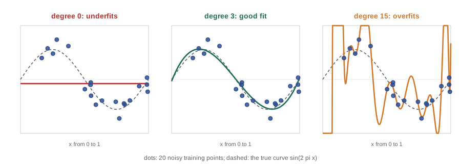
Consider fitting polynomials to 20 noisy observations of a smooth curve. A polynomial of degree 0 is a constant: it cannot follow the curve, so both its training and validation errors are large. That is underfitting, and its cause is a hypothesis class too restrictive to contain anything close to the truth. A polynomial of degree 15 can pass close to every one of the 20 points, so its training error is tiny, but between the points it swings wildly, and its validation error is enormous. That is overfitting, and its cause is a hypothesis class so flexible that the particular noise in this sample decides which function is chosen.

# Training and validation error of polynomial fits of increasing degree.
import numpy as np
rng = np.random.default_rng(367)
f = lambda x: np.sin(2 * np.pi * x)            # the unknown target function
def sample(n, noise=0.3):
    x = rng.uniform(0, 1, n)
    return x, f(x) + rng.normal(0, noise, n)

x_tr, y_tr = sample(20); x_va, y_va = sample(1000)
mse = lambda w, x, y: np.mean((np.polyval(w, x) - y) ** 2)
print("degree  train MSE  validation MSE")
for d in (0, 1, 3, 5, 9, 12, 15):
    w = np.polyfit(x_tr, y_tr, d)               # least-squares fit of a degree-d polynomial
    print(f"{d:6}  {mse(w, x_tr, y_tr):9.3f}  {mse(w, x_va, y_va):14.3f}")
print("noise variance (the floor):", 0.3 ** 2)

degree  train MSE  validation MSE
     0      0.549           0.579
     1      0.287           0.289
     3      0.069           0.094
     5      0.038           0.197
     9      0.031          60.176
    12      0.022      380223.173
    15      0.008     4586862.800
noise variance (the floor): 0.09

Training error falls steadily as the degree rises, because each larger class contains the smaller ones. Validation error is lowest at degree 3, rises at degree 5, and then explodes: by degree 9 the fitted curve swings so far between the training points that its validation error is hundreds of times the noise. No model can beat the noise variance of 0.09, and the best ones come within a few hundredths of it. The U shape of validation error against model complexity is the single most important picture in classical machine learning, and the next section explains it.

The bias–variance decomposition

Suppose the data are generated as \(y = f(x) + \varepsilon\), where f is the unknown true function and \(\varepsilon\) is noise with mean 0 and variance \(\sigma^2\), independent of x. A learning algorithm run on a random training set S produces a function \(\hat{h}_S\). Fix a test input x and ask for the expected squared error of the prediction, averaging over both the random training set and the noise in the test label. Write \(\bar{h}(x) = \mathbb{E}_S[\hat{h}_S(x)]\) for the average prediction over training sets.

Expand the error by adding and subtracting f(x) and \(\bar{h}(x)\):

Square the three terms and take expectations. The noise \(\varepsilon\) belongs to the test label, so it is independent of the training set and has mean zero; every cross term involving it vanishes. The middle term is a constant at fixed x. The last term has mean zero over S by definition of \(\bar{h}\), so the cross term between the constant and it also vanishes. Three squares remain:

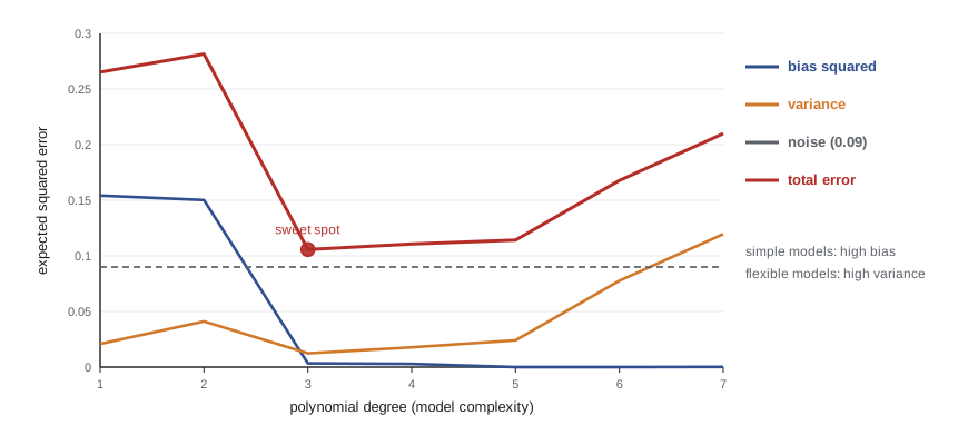
Each term has a meaning. The noise is irreducible: it is the Bayes error for squared loss. The squared bias measures how far the average prediction is from the truth; it is large when the hypothesis class cannot represent f, and it is the signature of underfitting. The variance measures how much the prediction changes from one training set to another; it is large when the class is so flexible that small changes in the data produce large changes in the fit, and it is the signature of overfitting. Averaging over x gives the same decomposition for the expected test error over the input distribution.

We can measure the two terms by simulation, because in an invented problem we know f and can draw as many training sets as we like. The program fits polynomials of several degrees to 500 independent training sets of 30 points each and averages.

# Estimating bias squared and variance by refitting on many independent training sets.
import numpy as np
rng = np.random.default_rng(42)
f = lambda x: np.sin(2 * np.pi * x)
sigma, n, trials = 0.3, 30, 500
x_grid = np.linspace(0.05, 0.95, 50)          # evaluate predictions at fixed test inputs
print("degree   bias^2  variance  noise  expected test MSE")
for d in (1, 3, 5, 7, 9):
    preds = np.empty((trials, x_grid.size))
    for t in range(trials):
        x = rng.uniform(0, 1, n); y = f(x) + rng.normal(0, sigma, n)
        preds[t] = np.polyval(np.polyfit(x, y, d), x_grid)
    mean_pred = preds.mean(axis=0)
    bias2 = np.mean((mean_pred - f(x_grid)) ** 2)
    var = np.mean(preds.var(axis=0))
    print(f"{d:6}  {bias2:7.3f}  {var:8.3f}  {sigma**2:5.2f}  {bias2 + var + sigma**2:17.3f}")

degree   bias^2  variance  noise  expected test MSE
     1    0.154     0.021   0.09              0.265
     3    0.003     0.013   0.09              0.106
     5    0.000     0.025   0.09              0.115
     7    0.000     0.103   0.09              0.193
     9    0.000     0.723   0.09              0.813

Degree 1 has large bias and small variance: a straight line cannot follow a sine wave, but every training set produces nearly the same line. By degree 5 the bias has vanished, and from there on extra flexibility buys nothing but variance, which grows slowly at first and then explosively at degree 9, where an occasional training set produces a fit that swings far from the data. Degree 3 sits near the sweet spot, with total expected error of about 0.11, close to the noise floor and close to the validation error that the previous program measured for its degree-3 fit.

The trade-off is not a law that every method obeys in the same way. Variance falls as the training set grows, so a model that overfits 20 points may be ideal for 20,000; this is why flexible models such as gradient-boosted trees and neural networks dominate when data are plentiful. Regularization, the subject of lesson 3, reduces variance at the cost of a little bias, by shrinking the fitted function toward something simple. Ensembles, the subject of lesson 7, reduce variance by averaging many fits. And very large neural networks show a phenomenon called double descent, in which test error rises near the point where the model can just interpolate the training data and then falls again as the model grows far beyond it; CMPUT-466 discusses why. The decomposition itself remains exactly true for squared loss; what changes is how bias and variance behave as a function of model size.

Probably approximately correct learning

The decomposition describes averages over hypothetical training sets. Learning theory instead asks for a guarantee about the one training set we have. Leslie Valiant's 1984 framework of probably approximately correct (PAC) learning, for which he received the 2010 Turing Award, phrases the guarantee with two tolerances: an accuracy parameter \(\varepsilon\) (approximately correct: true risk within \(\varepsilon\) of the target) and a confidence parameter \(\delta\) (probably: the guarantee may fail on an unlucky sample, but only with probability at most \(\delta\)). A hypothesis class is PAC-learnable if some algorithm achieves this for every distribution, with a sample size that grows only polynomially in \(1/\varepsilon\) and \(1/\delta\).

A bound for finite hypothesis classes

Start with the realizable case, in which some hypothesis in \(\mathcal{H}\) makes no errors. Call a hypothesis bad if its true risk exceeds \(\varepsilon\). A bad hypothesis agrees with a random example with probability less than \(1 - \varepsilon\), so it agrees with all n independent training examples with probability less than \((1 - \varepsilon)^n \le e^{-\varepsilon n}\). There are at most \(\lvert \mathcal{H} \rvert\) bad hypotheses, and by the union bound the probability that any of them has zero training error is less than \(\lvert \mathcal{H} \rvert e^{-\varepsilon n}\). Setting this at most \(\delta\) and solving gives the sample size that guarantees, with probability at least \(1 - \delta\), that every consistent hypothesis has risk at most \(\varepsilon\):

In the agnostic case, no hypothesis need be perfect, and we want the training error of every hypothesis to be close to its true error. For one fixed hypothesis, the training error is an average of n independent 0-1 variables, and Hoeffding's inequality bounds the chance that it deviates from its mean by more than \(\varepsilon\) by \(2e^{-2n\varepsilon^2}\). The union bound over the class gives, with probability at least \(1 - \delta\), simultaneously for all \(h \in \mathcal{H}\):

This uniform convergence is exactly what ERM needs. If every hypothesis's training error is within \(\varepsilon\) of its true error, then the hypothesis ERM picks has true risk at most \(2\varepsilon\) above the best in the class. Note the shape of the bound. The sample size grows with the logarithm of the class size, so even enormous finite classes are learnable; and it grows as \(1/\varepsilon^2\) in the agnostic case against \(1/\varepsilon\) in the realizable case, so noisy problems need many more examples for the same accuracy.

# Sample sizes from the finite-class bounds, and a check of the agnostic bound by simulation.
import math
import numpy as np

def realizable_n(H, eps, delta):
    """n such that, if some h in H is perfect, every h with zero training error has risk <= eps."""
    return math.ceil((math.log(H) + math.log(1 / delta)) / eps)

def agnostic_n(H, eps, delta):
    """n such that |true risk - training risk| <= eps for every h in H at once."""
    return math.ceil((math.log(H) + math.log(2 / delta)) / (2 * eps ** 2))

for H in (41, 10 ** 3, 10 ** 6, 2 ** 64):
    print(f"|H| = {H:<22} realizable n = {realizable_n(H, 0.05, 0.05):5}   agnostic n = {agnostic_n(H, 0.05, 0.05):6}")

# simulation: 41 threshold rules, n = 600; how often is the worst gap above the bound's eps?
rng = np.random.default_rng(7)
n, delta = 600, 0.05
eps = math.sqrt((math.log(41) + math.log(2 / delta)) / (2 * n))
x_big = rng.uniform(0, 40, 400_000)
y_big = (rng.uniform(size=x_big.size) < 1 / (1 + np.exp(-(x_big - 22) / 2.5))).astype(int)
true = np.array([np.mean((x_big >= t) != y_big) for t in range(41)])
worst = []
for _ in range(300):
    idx = rng.integers(0, x_big.size, n)
    emp = np.array([np.mean((x_big[idx] >= t) != y_big[idx]) for t in range(41)])
    worst.append(np.max(np.abs(emp - true)))
worst = np.array(worst)
print(f"bound eps = {eps:.3f}; mean worst gap = {worst.mean():.3f}; runs exceeding eps: {np.mean(worst > eps):.3f}")

|H| = 41                     realizable n =   135   agnostic n =   1481
|H| = 1000                   realizable n =   199   agnostic n =   2120
|H| = 1000000                realizable n =   337   agnostic n =   3501
|H| = 18446744073709551616   realizable n =   948   agnostic n =   9611
bound eps = 0.079; mean worst gap = 0.032; runs exceeding eps: 0.000

A class of \(2^{64}\) hypotheses, every function representable by a 64-bit description, needs only about seven times as many examples as a class of 41 in the realizable case, because the bound depends on \(\ln \lvert \mathcal{H} \rvert\), essentially the number of bits needed to name a hypothesis. The simulation shows the other side of worst-case bounds: the guarantee held in every run, but the typical worst gap was well under half of \(\varepsilon\). The union bound treats the 41 thresholds as if their errors were independent, when in fact neighboring thresholds make nearly the same mistakes. Bounds of this kind are valuable for the dependence they reveal, not for their constants.

Infinite classes and the VC dimension

Most useful hypothesis classes are infinite: a linear classifier has real-valued weights. The finite bound is useless for them, yet linear classifiers clearly can be learned. Vladimir Vapnik and Alexey Chervonenkis showed in the early 1970s that what matters is not the number of hypotheses but how many different ways the class can label a set of points. A class \(\mathcal{H}\) shatters a set of m points if, for every one of the \(2^m\) possible labellings, some hypothesis in \(\mathcal{H}\) produces it. The VC dimension of \(\mathcal{H}\) is the size of the largest set it can shatter.

The last row is a useful warning: the VC dimension is not the number of parameters, even though for many classes the two are close. The fundamental theorem of statistical learning says that a class is PAC-learnable if and only if its VC dimension d is finite, and that the agnostic sample size needed is proportional to \((d + \ln(1/\delta)) / \varepsilon^2\). A standard form of the resulting generalization bound states that, with probability at least \(1 - \delta\), for all \(h \in \mathcal{H}\),

The precise constants differ between textbooks; the shape is what matters. The gap shrinks like \(\sqrt{d/n}\) up to a logarithm, so to keep it fixed the number of examples must grow in proportion to the VC dimension. A rough rule of thumb inherited from this result, ten examples per parameter, is crude but has the right flavor for simple models. It is badly wrong for modern overparameterized networks, which generalize well with far more parameters than examples, for reasons that worst-case VC theory does not capture; margin-based bounds (lesson 5), norm-based bounds and stability arguments come closer.

Structural risk minimization and model selection

The bounds suggest a principle for choosing a hypothesis class. Arrange classes in a nested sequence \(\mathcal{H}_1 \subset \mathcal{H}_2 \subset \cdots\) of increasing capacity, such as polynomials of increasing degree. Training error falls along the sequence, while the complexity term of the bound rises. Vapnik's structural risk minimization chooses the class that minimizes their sum. In practice the complexity term is too loose to use directly, and its job is done instead by an estimate of test error on validation data, or by a penalty added to the training loss. Regularized learning, \(\min_h \hat{R}_S(h) + \lambda \Omega(h)\) with a complexity penalty \(\Omega\), is the continuous version of the same idea, and lesson 3 develops it for linear models. Information criteria such as AIC and BIC, which STAT-151 met for regression, are other penalized-likelihood versions.

Whichever approach is used, the lesson of this chapter is the same: model capacity must be matched to the amount of data and the amount of noise. With little data, prefer simple models or strong regularization; with abundant data, flexible models become affordable. And always estimate generalization on data that played no part in fitting.

Worked examples