
CIV-470 · Lesson 2 of 12 · 19 min
Reservoir storage and yield
Streamflow is generous in spring and mean in late summer and winter. A reservoir moves water from the times of plenty to the times of need, and the central question of reservoir design is how much storage is needed to supply a given draft reliably. Kestrel Lake is a natural lake raised by a small dam built in 1958. Its active storage, the volume between the spillway crest and the lowest level the intake and the shoreline can tolerate, is what supplies the co-op and the minimum release to the creek. In this lesson the team checks whether that storage can meet the 25-year demand from lesson 1.
Reservoir storage zones
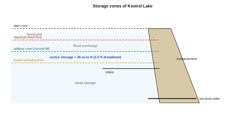
A reservoir's volume is divided into zones. Dead storage lies below the lowest outlet and cannot be released; it also collects sediment, the subject of lesson 3. Active or conservation storage lies between the lowest operating level and the normal full level, usually the spillway crest; it supplies the draft. Flood storage lies above the normal full level, up to the maximum design flood level; it is filled temporarily during floods and empties through the spillway and outlets. Freeboard is the height of the dam crest above the maximum flood level, provided for waves, wind setup, settlement and uncertainty.
The relation between water level, surface area and volume is the reservoir's stage-area-capacity curve, built from a bathymetric survey and the surrounding topography. Kestrel Lake has a surface area of about 23.5 acres at the spillway crest, and the lakeshore residents and the intake limit the drawdown to 2.0 ft. Because the lake's sides are steep near the shoreline, the area changes little over that range, and the active storage is close to area times drawdown: about 46 acre-ft.
The mass curve and the sequent peak method
The classical tool is Rippl's mass curve, introduced in the 1880s: plot the cumulative inflow against time, and the cumulative demand on the same axes. Wherever the demand line is steeper than the inflow curve the reservoir is drawing down; the largest cumulative deficit between a peak of the inflow curve and a later trough defines the storage needed. The sequent peak method does the same arithmetic in a form suited to a spreadsheet or code. Starting with zero, each period adds the deficit (draft minus inflow) to a running total that cannot fall below zero:
The record is analyzed twice in succession, so that a deficit that begins near the end of the record and would continue into the next year is captured. The method assumes the future will repeat the record, it ignores evaporation and seepage unless they are added to the draft, and it gives the storage that would just have avoided any shortage in the record. A longer record, or a synthetic record generated from the statistics of the observed one, gives a more reliable answer, because the critical drought in a short record may be milder than the droughts the reservoir will face.
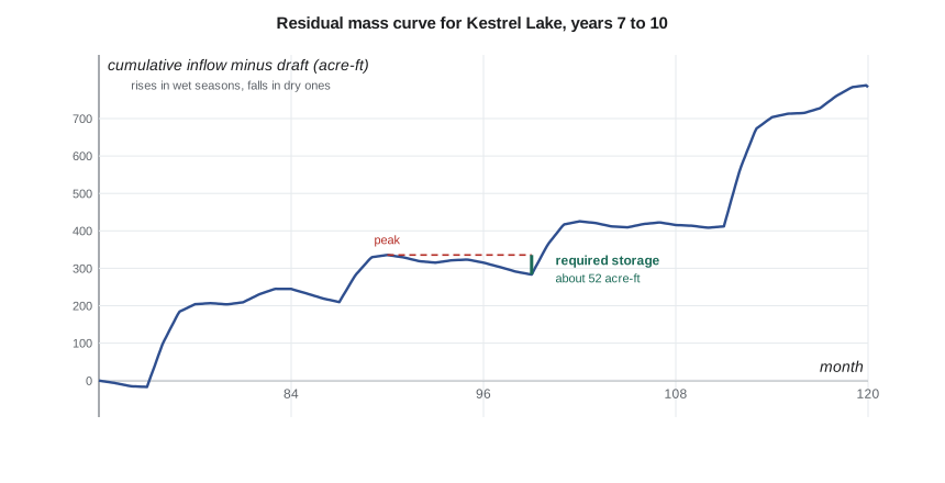
Subtracting the cumulative draft from the cumulative inflow gives the residual mass curve, which shows the same information more clearly: it rises when inflow exceeds the draft and falls when the reservoir is drawing down, and the required storage is the largest fall from any peak to a later trough. That is exactly what the sequent peak calculation finds.
The draft and the environmental release
The draft on Kestrel Lake has two parts. The co-op's year-25 average demand is about 103 gpm, from lesson 1. The second part is the minimum release to the creek, which keeps the reach below the dam wet for brook trout and other aquatic life in summer and under the ice in winter. Environmental flows are a field of their own: simple methods set the release as a fraction of the mean annual flow, often 10 to 30 %, while habitat methods model how depth and velocity in the reach change with flow. The co-op's existing approval sets a minimum of 79 gpm, about 20 % of the mean inflow, and the fisheries agency has asked whether a larger release in late summer is possible.
The total draft of 182 gpm is 46 % of the mean inflow to the lake of 0.88 cfs. That is a high development ratio. As a rule, the storage needed rises slowly while the draft is a small fraction of the mean flow and very steeply as the draft approaches the mean, because ever-longer runs of below-average years must be bridged.
Reliability and simulation
No finite reservoir is perfectly reliable. Reliability can be measured as the fraction of periods with no shortage (time-based reliability), the fraction of the demand supplied (volumetric reliability), or the probability of no failure during the design life. Resilience describes how quickly the system recovers from a shortage, and vulnerability how deep shortages are. A water supply reservoir for a community is commonly designed for a drought of about 1-in-50 or 1-in-100 year severity, with drought restrictions as the planned response to anything worse.
Simulation is the tool for these measures. The reservoir is operated month by month through the record or through many synthetic records: storage is updated with inflow minus draft, any storage above full is spilled, and any shortfall is recorded. Simulation can include rules that a sequent peak calculation cannot, such as cutting the draft when the lake falls below a trigger level, or varying the environmental release with the season.
# Kestrel Lake: sequent peak storage, simulation and reliability
UNITS = "US"
SI = UNITS == "SI"
# monthly inflow (m3/s) for a 10-year synthetic record: a seasonal pattern times a year factor
season = [0.012, 0.010, 0.015, 0.095, 0.070, 0.030, 0.018, 0.014, 0.020, 0.030, 0.026, 0.016]
years = [1.00, 0.82, 1.15, 0.64, 0.92, 1.25, 0.71, 0.48, 0.52, 0.88]
days = [31, 28, 31, 30, 31, 30, 31, 31, 30, 31, 30, 31]
Q = [s * f for f in years for s in season]
D = [d * 86400 for _ in years for d in days]                 # seconds in each month
demand = 0.0065 + 0.0050                                     # year-25 supply 6.5 L/s + environmental release 5.0 L/s
mean_in = sum(q * d for q, d in zip(Q, D)) / sum(D)
print(f"Mean inflow {mean_in*1000:.1f} L/s; draft {demand*1000:.1f} L/s ({demand/mean_in:.0%} of the mean)" if SI else
      f"Mean inflow {mean_in*35.315:.2f} cfs; draft {demand*15850:.0f} gpm ({demand/mean_in:.0%} of the mean)")

def sequent_peak(draft):
    K, Kmax = 0.0, 0.0
    for q, d in zip(Q + Q, D + D):                            # record repeated twice, as the method requires
        K = max(0.0, K + (draft - q) * d)
        Kmax = max(Kmax, K)
    return Kmax
need = sequent_peak(demand)
cv = lambda v: f"{v/1000:,.0f} thousand m3" if SI else f"{v/1233.5:,.0f} acre-ft"
print(f"Sequent peak storage for the draft: {cv(need)}")
for frac in (0.3, 0.4, 0.5, 0.6):
    print(f"  draft {frac:.0%} of mean -> storage {cv(sequent_peak(frac * mean_in))}")

S_active = 9.5e4 * 0.60                                      # 9.5 ha lake drawn down at most 0.60 m: active storage, m3
def simulate(S_cap, draft):
    S, fails, low = S_cap, 0, S_cap
    for q, d in zip(Q, D):
        S = S + (q - draft) * d
        if S > S_cap: S = S_cap                              # spill
        if S < 0: S = 0; fails += 1                          # shortage in this month
        low = min(low, S)
    return fails, low
f, low = simulate(S_active, demand)
print(f"\nSimulation with {cv(S_active)} of active storage: shortage in {f} of {len(Q)} months; "
      f"reliability {1 - f/len(Q):.1%}; lowest storage {cv(low)}")
f2, low2 = simulate(S_active, 0.0065 + 0.0050 * 1.6)
print(f"With the environmental release raised 60 %: shortage in {f2} months; reliability {1 - f2/len(Q):.1%}")Mean inflow 0.88 cfs; draft 182 gpm (46% of the mean) Sequent peak storage for the draft: 52 acre-ft draft 30% of mean -> storage 9 acre-ft draft 40% of mean -> storage 27 acre-ft draft 50% of mean -> storage 70 acre-ft draft 60% of mean -> storage 119 acre-ft Simulation with 46 acre-ft of active storage: shortage in 1 of 120 months; reliability 99.2%; lowest storage 0 acre-ft With the environmental release raised 60 %: shortage in 9 months; reliability 92.5%
Reading the results
The sequent peak storage for the 182 gpm draft is about 52 acre-ft, more than the 46 acre-ft of active storage the lake can give. The simulation confirms it: through the ten-year record the lake meets the draft in 119 of 120 months and runs dry for one month at the end of the two-year drought in years 8 and 9. If the DNR fisheries staff's request for a 60 % higher late-summer release were applied all year, shortages would occur in 9 months, a reliability of only 92.5 %. The storage-yield relation shows the cause: storage needs rise from about 27 acre-ft at a draft of 40 % of the mean flow to 70 acre-ft at 50 %. The lake is near the steep part of the curve.
Three responses are possible: raise the dam to add storage, which brings dam safety and shoreline issues; cut the draft in droughts with restrictions; or add a second source. The team carries the third forward to lesson 11, where wells in the confined aquifer are tested as a drought backup.
Worked problem
Sequent peak by hand
A small reservoir has the following inflows in four successive seasons, in thousands of acre-ft per season: 120, 40, 25, 95, and the record repeats. The draft is 60 per season. Find the required storage.
Show solution
- Season 1: \(K = \max(0, 0 + 60 - 120) = 0\).
- Season 2: \(K = \max(0, 0 + 60 - 40) = 20\).
- Season 3: \(K = \max(0, 20 + 60 - 25) = 55\).
- Season 4: \(K = \max(0, 55 + 60 - 95) = 20\).
- Repeat: season 1 gives \(\max(0, 20 + 60 - 120) = 0\), and the pattern repeats.
- \[S_{\text{required}} = \max K_t = 55\]
Answer: A storage of 55 thousand acre-ft bridges the two dry seasons; the mean inflow (70) exceeds the draft (60), so the reservoir refills.
| Draft (% of mean inflow) | Required storage (acre-ft) | Comment |
|---|---|---|
| 30 | 9 | well within active storage |
| 40 | 27 | within active storage |
| 46 (year-25 need) | 52 | exceeds the active storage |
| 50 | 70 | needs a higher dam or a second source |
| 60 | 119 | impractical |
Losses and other refinements
Evaporation from the lake surface and seepage through and under the dam reduce the water available. Over a small, deep lake in a cool climate, evaporation in summer is roughly equal to the precipitation falling on the lake, but in a dry month the net loss can be 1 to 1.5 in. over the surface, a few thousand cubic meters for Kestrel Lake. A full study adds net evaporation to the draft month by month. Ice cover in winter reduces evaporation but also reduces the usable depth near the intake, and the winter low-flow period, when inflow is small and the release must continue, is often the critical season in northern reservoirs, not late summer.
Operating rules matter as much as size. Rule curves define target levels through the year, and drought triggers define when restrictions start. A reservoir that begins restrictions early, when storage falls below a trigger, can reduce the depth of shortages greatly at the cost of more frequent mild restrictions. These rules are tested by simulation, ideally with many synthetic sequences that include droughts longer than the observed record.
Practical points
- Define active storage from the operating limits: the intake level, shoreline uses and fish habitat, not just the geometry.
- Run the sequent peak over the record twice in succession.
- Expect storage needs to rise steeply as the draft approaches the mean flow.
- Add net evaporation and seepage to the draft in dry months.
- Use simulation to test operating rules, environmental releases and droughts longer than the record.
Common mistakes
MistakeSizing storage from the mean annual inflow alone.
InsteadStorage depends on the sequence of dry periods, not the mean.
MistakeUsing a short record and assuming its worst drought is the design drought.
InsteadExtend the record or generate synthetic sequences; short records rarely include the critical drought.
MistakeForgetting the environmental release in the draft.
InsteadThe release is a firm draft like any other, often with seasonal requirements.
MistakeAssuming the whole lake volume is usable.
InsteadOnly the active storage between operating limits supplies the draft.
Summary and key terms
- Reservoir volume is divided into dead, active and flood storage, with freeboard above.
- The mass curve and the sequent peak method give the storage that would have met a draft through the record.
- Storage needs rise steeply as the draft approaches the mean inflow.
- Kestrel Lake's active storage of 46 acre-ft is less than the 52 acre-ft needed for the year-25 draft of 182 gpm.
- Simulation gives reliability, resilience and vulnerability and can include operating rules.
- A second source, restrictions or more storage can close the gap; the plan tests wells.
- Active storage
- The volume between the lowest operating level and the normal full level that supplies the draft.
- Dead storage
- Volume below the lowest outlet, which cannot be released.
- Draft
- The rate at which water is withdrawn or released from a reservoir.
- Mass curve
- A plot of cumulative inflow against time, used with a cumulative demand line to find storage.
- Sequent peak method
- A running-deficit calculation over a repeated record that gives the required storage.
- Firm yield
- The largest draft that a reservoir could have supplied without shortage through the record.
- Reliability
- The fraction of time, or of demand, for which the reservoir meets the draft.
- Environmental flow
- A release that sustains the ecological health of the stream below a dam.
Practice problems
Work each problem on paper first, then reveal the answer to check.
Inflows in five periods are 50, 20, 10, 15, 70 and the draft is 30 in each. Find the storage by sequent peak, repeating the record.
Show answer
K: 0, 10, 30, 45, 5; repeat: 0, 10, 30, 45, 5. Required storage 45.
A lake has an area of 30 acres and can be drawn down 2.6 ft. Estimate its active storage.
Show answer
About 78 acre-ft.
Why does the storage needed rise steeply as the draft approaches the mean flow?
Show answer
Longer and longer runs of below-average years must be bridged, and the reservoir has less surplus to refill between them.
Give one advantage of simulation over the sequent peak method.
Show answer
Simulation can apply operating rules, drought restrictions and seasonal releases, and report reliability measures.
Lesson quiz · 5 questions
Score 60% or more to complete this lesson.
Create a free account to save your progress, take quizzes and earn a certificate.