
CIV-470 · Lesson 11 of 12 · 19 min
Groundwater and conjunctive use
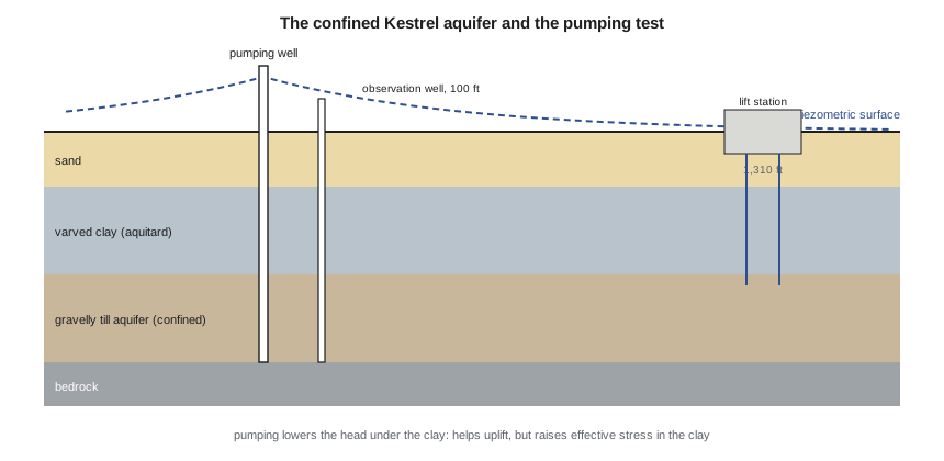
Lesson 2 left the co-op short of water in the worst drought of the record: Kestrel Lake's active storage cannot carry the year-25 draft through two dry years. The cheapest second source is beneath the watershed. The ground model from CIV-340, sand over varved clay over an artesian till, includes a layer of gravelly till at depth that the CIV-440 relief wells tapped at the lift station, where its water pressure rose above the ground. If that aquifer can yield a few liters a second through a dry summer, wells can back up the lake: the combined use of surface water and groundwater called conjunctive use. This lesson tests the aquifer and checks what pumping it would do to its neighbors.
Aquifers and their properties
An aquifer is a saturated formation that stores and transmits enough water to supply wells. An unconfined aquifer has a free water table open to the atmosphere through the soil above it; a confined aquifer lies beneath a layer of low permeability, an aquitard, and its water is under pressure, so the water level in a well rises above the top of the aquifer, and above the ground in an artesian or flowing well. The Kestrel till aquifer is confined by the varved clay, and its head stands about 5 ft above the ground near the creek.
Two properties describe an aquifer. Transmissivity \(T\), the product of hydraulic conductivity and saturated thickness, measures how easily water moves through the full thickness. Storativity \(S\) measures how much water the aquifer releases per unit area per unit decline in head. In a confined aquifer, water comes from compression of the aquifer and expansion of the water, so \(S\) is small, typically \(10^{-5}\) to \(10^{-3}\); in an unconfined aquifer the pores drain, and the specific yield is typically 0.05 to 0.3. That difference is why pumping a confined aquifer spreads its effects much farther, much faster, than pumping an unconfined one.
Flow to a well: Theis
When a well starts pumping a confined aquifer at a steady rate, the head falls around it in a widening cone of depression. Theis, in 1935, solved the problem for an ideal confined aquifer, infinite in extent, uniform, with all water released from storage:
where \(s\) is the drawdown at distance \(r\) and time \(t\), and \(W(u)\) is the well function, a standard integral evaluated from tables or a series. Drawdown grows with the pumping rate and with time, and falls with distance and with transmissivity. The cone keeps expanding as long as pumping continues, until it reaches a boundary that supplies water, such as a lake or stream, or until leakage through the confining layer balances the pumping.
The Cooper-Jacob straight line
For small values of \(u\), late in a test or close to the well, the well function is closely approximated by \(W(u) \approx -0.5772 - \ln u\). The drawdown then plots as a straight line against the logarithm of time, which gives a simple way to find the aquifer properties from a pumping test:
where \(\Delta s\) is the drawdown per log cycle of time and \(t_0\) the time at which the straight line crosses zero drawdown. The approximation holds when \(u\) is below about 0.05; the analyst checks this after finding \(T\) and \(S\), and fits the line only to the data that satisfy it. Departures from the straight line also carry information: flattening suggests leakage or a recharge boundary such as the lake, and steepening suggests a barrier such as the edge of the aquifer.
The co-op's hydrogeologist ran a 24-hour test on a new well near Kestrel Lake at 95 gpm, recording drawdown in an observation well 100 ft away. A test of this kind, with a report on interference with other water users, supports the application for a water appropriation permit.
# Confined till-gravel aquifer: pumping test (Cooper-Jacob), Theis predictions and conjunctive use
from math import log10, log, exp, pi
UNITS = "US"
SI = UNITS == "SI"
Q = 6.0 / 1000                                 # test pumping rate, m3/s (6 L/s)
r_obs = 30.0                                   # observation well distance, m
t_min = [10, 20, 50, 100, 200, 500, 1000, 1440]
s_obs = [0.62, 0.89, 1.24, 1.51, 1.78, 2.14, 2.41, 2.55]   # drawdown, m (field record, rounded)
# straight-line fit of s against log10(t) on the late data (u < 0.05)
xs = [log10(t) for t in t_min[3:]]; ys = s_obs[3:]
n = len(xs); mx = sum(xs) / n; my = sum(ys) / n
slope = sum((x - mx) * (y - my) for x, y in zip(xs, ys)) / sum((x - mx) ** 2 for x in xs)
t0 = 10 ** (mx - my / slope) * 60              # time of zero drawdown on the line, s
T = 2.30 * Q / (4 * pi * slope)
Sc = 2.25 * T * t0 / r_obs ** 2
if SI:
    print(f"Drawdown per log cycle {slope:.3f} m; t0 = {t0:.0f} s")
    print(f"Transmissivity T = 2.30 Q / (4 pi ds) = {T*86400:.1f} m2/d; storativity S = 2.25 T t0 / r^2 = {Sc:.1e}")
else:
    print(f"Drawdown per log cycle {slope/0.3048:.3f} ft; t0 = {t0:.0f} s")
    print(f"Transmissivity T = 264 Q / ds = {T*86400/0.3048**2*7.48:,.0f} gpd/ft; storativity S = 0.3 T t0 / r^2 = {Sc:.1e}")
u_last = r_obs ** 2 * Sc / (4 * T * t_min[-1] * 60)
print(f"Check: u at the end of the test = {u_last:.4f} (the straight line needs u < about 0.05)")

def W(u, terms=40):                             # Theis well function by its series
    s, term = -0.5772156649 - log(u), 1.0
    for k in range(1, terms):
        term *= -u / k
        s -= term / k
    return s
# long-term pumping at 4 L/s from two wells; drawdown at the lift station relief wells 400 m away
for days in (30, 120):
    t = days * 86400
    sd = 2 * 0.004 / (4 * pi * T) * W(400 ** 2 * Sc / (4 * T * t))
    print(f"After {days:3d} days at 2 x 4 L/s: drawdown at the lift station (400 m) {sd:.2f} m" if SI else
          f"After {days:3d} days at 2 x 63 gpm: drawdown at the lift station (1,310 ft) {sd/0.3048:.2f} ft")
# conjunctive use: wells cover what the reservoir cannot in a dry year
need = [11.5] * 12                              # supply + environmental release, L/s
avail = [8.2, 7.1, 9.0, 11.5, 11.5, 11.5, 10.4, 8.6, 9.8, 11.5, 11.5, 9.3]    # reservoir in the dry year, L/s
gap = [max(0.0, a - b) for a, b in zip(need, avail)]
print(f"\nDry year: the wells must supply {sum(g * 30.4 * 86.4 for g in gap):,.0f} m3, peak {max(gap):.1f} L/s" if SI else
f"\nDry year: the wells must supply {sum(g * 30.4 * 86.4 for g in gap)*264.17/1e6:,.2f} million gal, peak {max(gap)*15.85:.0f} gpm")Drawdown per log cycle 2.949 ft; t0 = 125 s Transmissivity T = 264 Q / ds = 8,498 gpd/ft; storativity S = 0.3 T t0 / r^2 = 3.8e-04 Check: u at the end of the test = 0.0008 (the straight line needs u < about 0.05) After 30 days at 2 x 63 gpm: drawdown at the lift station (1,310 ft) 8.14 ft After 120 days at 2 x 63 gpm: drawdown at the lift station (1,310 ft) 10.50 ft Dry year: the wells must supply 12.56 million gal, peak 70 gpm
Reading the results
The late test data fall on a straight line with 2.95 ft of drawdown per log cycle, giving a transmissivity of about 8,500 gpd/ft and a storativity of \(3.8 \times 10^{-4}\), typical of a confined gravelly till. The value of \(u\) at the end of the test is 0.0008, so the straight-line method is valid. In a repeat of the dry year of lesson 2, the reservoir falls short by up to 70 gpm and the wells must supply about 12.6 million gallons over the year, well within the capacity of two wells at 63 gpm each.
The Theis prediction carries a warning. Two wells pumping 63 gpm each would lower the head at the lift station, 1,310 ft away, by about 8 ft after a month and 10.5 ft after four months. At first sight that helps the uplift problem of CIV-440, where the artesian pressure threatened the base of the wet well excavation. But the head drop also raises the effective stress in the varved clay above the aquifer, and Dr. Kowalczyk's first estimate is that a season of that drawdown could consolidate the clay under the operations center by 0.4 to 1.2 in., enough to matter to the floor slabs and buried pipes designed in CIV-341.
Theis assumes no leakage, so the real drawdown will be less as water seeps down through the clay and as the cone reaches the lake, but the risk is real. The plan therefore limits the wells to the gap rate in drought months, rather than full capacity, places them at the far end of the aquifer from the operations center, adds piezometers between the wells and the lift station with a trigger level for reducing pumping, and requires a longer test with leakage analysis before the permit application.
Worked problem
Cooper-Jacob by hand
A well pumps 79 gpm from a confined aquifer. In an observation well 164 ft away, the late drawdowns plot on a line that falls 2.46 ft per log cycle and crosses zero drawdown at 3.0 minutes. Find \(T\) and \(S\).
Show solution
- In US practice, \(T = 264\,Q/\Delta s\) with \(Q\) in gpm, \(\Delta s\) in ft and \(T\) in gpd/ft:
- \[T = \frac{264 \times 79}{2.46} = 8{,}480\ \text{gpd/ft}\]
- \[S = \frac{0.3\,T\,t_0}{r^2} = \frac{0.3 \times 8{,}480 \times (3.0/1440)}{164^2} = 2.0 \times 10^{-4}\]
Answer: The storativity confirms a confined aquifer; the result should be checked by computing \(u\) at the times used.
Wellhead protection and well construction
Water taken from wells must be protected from contamination. Wellhead protection areas are mapped around municipal and community wells from the time water takes to travel to the well, and land uses that could contaminate the aquifer, such as fuel storage, salt storage and certain industries, are restricted within them. Wells themselves must be built so that surface water cannot run down the outside of the casing into the aquifer, with grouted casings, sealed tops above flood level and proper decommissioning of old wells.
In Minnesota, the Department of Health runs the wellhead protection program for public water supplies, delineating drinking water supply management areas, commonly based on a 10-year time of travel, and working with communities on plans to manage contamination sources in them. Well construction and sealing follow the Minnesota Well Code. The operations center's salt shed must lie outside the wellhead protection area of any co-op well.
| Operation | Lake | Wells | Comment |
|---|---|---|---|
| Normal years | full draft, 182 gpm | off, exercised monthly | lake refills each spring |
| Lake below trigger level | reduced draft | gap rate, up to 70 gpm | piezometers checked weekly |
| Severe drought | minimum release only | both wells, up to 126 gpm | restrictions on lawn watering |
| Piezometer trigger reached | as above | reduce pumping | protects the clay under the operations center |
Conjunctive use
Conjunctive use combines the strengths of the two sources. Surface water is plentiful in most years but unreliable in droughts; groundwater is limited in rate but steady, and the aquifer's large storage carries over from year to year. Operating rules use the lake when it is full and draw on the wells when the lake falls below a trigger, letting the aquifer recover in wet years. The same idea applies at the scale of river basins, where reservoirs and aquifers are operated together, and where managed aquifer recharge stores surplus surface water underground. Climate change strengthens the case for conjunctive systems, because droughts are expected to become more variable while aquifers buffer short-term swings.
Practical points
- Identify whether an aquifer is confined or unconfined; storativity changes the reach of pumping effects by orders of magnitude.
- Check \(u\) before using the Cooper-Jacob straight line, and read departures from it as information about boundaries.
- Predict interference with other wells, springs, streams and structures before pumping starts.
- Remember that lowering heads under compressible clay can cause settlement.
- Protect wellheads by construction and by land use controls in time-of-travel areas.
Common mistakes
MistakeFitting the Cooper-Jacob line to early data.
InsteadUse only data with \(u\) below about 0.05.
MistakeAssuming pumping effects are local because the well is small.
InsteadIn a confined aquifer the cone spreads far and fast; compute it.
MistakeTreating groundwater as unlimited because the aquifer is large.
InsteadThe sustainable yield depends on recharge, interference and environmental effects.
MistakeOverlooking the effect of drawdown on overlying clay.
InsteadIncreased effective stress consolidates clay and can damage structures.
Summary and key terms
- Confined aquifers lie beneath aquitards and have small storativity; unconfined aquifers have a water table and large specific yield.
- The Theis solution gives drawdown around a well; the Cooper-Jacob line gives \(T\) and \(S\) from a pumping test.
- The Kestrel till aquifer has \(T \approx 8{,}500\) gpd/ft and \(S \approx 3.8 \times 10^{-4}\); dry-year needs are about 12.6 million gallons.
- Drawdown at the lift station could consolidate the varved clay, so pumping is limited and monitored.
- Wellhead protection areas and proper well construction protect the supply.
- Conjunctive use draws on the lake in normal years and the wells in droughts.
- Aquifer
- A saturated formation that stores and transmits enough water to supply wells.
- Aquitard
- A layer of low permeability that restricts groundwater flow.
- Confined aquifer
- An aquifer beneath an aquitard, in which water is under pressure.
- Transmissivity
- The rate at which water passes through the full thickness of an aquifer under a unit gradient.
- Storativity
- The volume of water released from storage per unit area per unit decline in head.
- Cone of depression
- The lowered piezometric surface around a pumping well.
- Wellhead protection area
- The land around a well within which contaminants could reach it in a defined time.
- Conjunctive use
- The coordinated use of surface water and groundwater.
Practice problems
Work each problem on paper first, then reveal the answer to check.
Find \(u\) for \(r = 330 ft\), \(S = 2 \times 10^{-4}\), \(T = 8,000 gpd/ft\) and \(t = 1\) day. Is the Cooper-Jacob method valid?
Show answer
Convert \(T\) to about 1,070 ft²/d: \(u = 330^2(2 \times 10^{-4})/(4 \times 1{,}070) = 0.005\); yes.
With \(W(u) = 4.0\), find the drawdown for \(Q = 79 gpm\) and \(T = 8,000 gpd/ft\).
Show answer
Using \(s = 114.6\,Q\,W(u)/T\): \(s = 114.6 \times 79 \times 4.0/8{,}000 = 4.5\) ft.
Why does a cone of depression spread farther in a confined aquifer than in an unconfined one?
Show answer
The storativity is much smaller, so less water is released per unit decline and the head must fall over a larger area.
Name two signs in a pumping test that indicate a boundary.
Show answer
Flattening of the drawdown curve suggests a recharge boundary or leakage; steepening suggests a barrier boundary.
Lesson quiz · 5 questions
Score 60% or more to complete this lesson.
Create a free account to save your progress, take quizzes and earn a certificate.