
CIV-280 · Lesson 10 of 12 · 22 min
Air pollution meteorology and dispersion
The same emission can be harmless on a windy afternoon and dangerous on a still winter night. What happens to pollution after it leaves a stack or tailpipe depends on the weather: how fast the wind blows, which way, and above all how readily the air near the ground mixes vertically. In December 1952 a temperature inversion trapped coal smoke over London for five days and caused thousands of deaths; in valleys and prairie cities today, winter inversions still hold wood smoke and vehicle exhaust close to the ground. This lesson covers the structure of the lower atmosphere, lapse rates and stability, plume behavior, the mixing height, wind roses, and the Gaussian plume model used to estimate concentrations downwind of a source. It ends by applying the model to the asphalt plant from lesson 9.
The lower atmosphere
Weather and nearly all air pollution occur in the troposphere, the lowest 10 to 16 km of the atmosphere, where temperature usually falls with height. Within it, the atmospheric boundary layer, typically a few hundred meters deep at night and one to three kilometers deep on a sunny afternoon, is the layer directly affected by the ground: heated by it during the day, cooled by it at night, and slowed by friction with buildings, trees and terrain. Pollutants released near the ground mix through the boundary layer, so its depth controls how much air is available to dilute them.
Lapse rates and stability
A parcel of air that rises expands as the pressure around it falls, and expansion cools it. If the parcel exchanges no heat with its surroundings, it cools at the dry adiabatic lapse rate of about 9.8 °C per kilometer, or roughly 1 °C per 100 m. Whether the parcel keeps rising or sinks back depends on how its temperature compares with the actual temperature of the surrounding air, which follows the environmental lapse rate measured by weather balloons and towers.
| Environmental lapse rate | Stability | What a displaced parcel does | Effect on pollution |
|---|---|---|---|
| Temperature falls faster than 9.8 °C/km (superadiabatic) | Unstable | Keeps moving away from its starting level | Strong vertical mixing; good dilution but plumes may loop to the ground |
| Temperature falls at about 9.8 °C/km | Neutral | Stays where it is put | Moderate mixing |
| Temperature falls slower than 9.8 °C/km | Stable | Returns toward its starting level | Weak vertical mixing |
| Temperature rises with height (inversion) | Very stable | Strongly pushed back | Pollution trapped; poor dilution |
Stability changes over the day. On a sunny afternoon the ground heats the air above it, producing an unstable, well-mixed boundary layer. On a clear, calm night the ground radiates heat to space and cools the air above it, forming a surface inversion that can be a few tens to a few hundred meters deep. Overcast and windy conditions push the atmosphere toward neutral. Prairie winters, with long nights, snow cover that reflects sunlight and frequent high-pressure systems, produce strong and persistent inversions that can last for days, especially in river valleys.
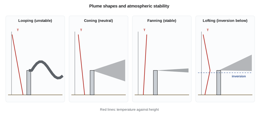
Plume shapes show the stability at a glance. A looping plume in unstable air can bring high concentrations to the ground briefly and close to the stack. A coning plume in neutral air spreads evenly. A fanning plume in stable air spreads sideways but hardly at all vertically, so it travels a long way without touching the ground. The most dangerous pattern is fumigation, which occurs on a morning after a night-time inversion: the sun heats the ground and erodes the inversion from below, and the pollution that accumulated aloft overnight in a fanning plume is suddenly mixed down to the ground.
Mixing height and wind
The mixing height is the depth of the layer within which pollutants mix vigorously, usually the top of the boundary layer, often capped by an elevated inversion that acts like a lid. Multiplying the mixing height by the average wind speed in the mixed layer gives the ventilation coefficient, an index of the atmosphere's capacity to dilute pollution. Low ventilation coefficients, typical of winter mornings and of valleys, mean poor dispersion, and many jurisdictions use them to decide when open burning or prescribed fires may proceed.
Wind speed dilutes pollution directly: doubling the wind speed doubles the volume of air passing a source each second and roughly halves the concentration downwind. Wind direction decides who is affected. A wind rose summarizes years of hourly wind data as a star-shaped chart showing how often the wind blows from each direction and at what speeds. On the prairies, winds from the northwest and south are common, so a new industrial site is best placed where the prevailing winds carry its emissions away from homes, schools and hospitals.
The Gaussian plume model
For a continuous point source such as a stack, the most widely used dispersion model assumes that the plume travels downwind with the mean wind and spreads sideways and vertically so that its concentration has a Gaussian, or bell-shaped, distribution in both directions. The spread grows with distance and is larger in unstable air. With the ground treated as a perfect reflector, which is expressed by adding an image source below the ground, the concentration at a point x downwind, y crosswind and z above the ground is:
Q is the emission rate in g/s, u the wind speed at stack height in m/s, H the effective stack height in m, and σ_y and σ_z the horizontal and vertical dispersion coefficients in m. For the concentration at ground level directly beneath the plume centerline (y = 0, z = 0), the equation simplifies to:
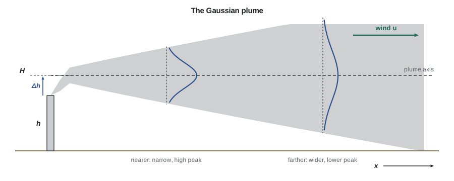
The effective stack height is the physical stack height plus the plume rise, the extra height a plume gains because it leaves the stack with upward momentum and because it is hotter and more buoyant than the surrounding air. Plume rise is estimated with empirical equations such as those of Gary Briggs, and on hot, fast exhausts it can be larger than the stack itself. A taller effective height gives the plume more distance to spread before it reaches the ground, which lowers the maximum ground-level concentration and moves it farther downwind.
The dispersion coefficients depend on distance and on stability. A common scheme groups weather into six Pasquill-Gifford stability classes from A (very unstable, sunny with light winds) to F (very stable, clear nights with light winds), with D for neutral, overcast or windy conditions. For hand calculations, σ_y and σ_z are read from charts or computed with power-law fits to those charts. The fits below, with x in kilometers and σ in meters, are a standard textbook set for distances under 1 km:
| Class | σ_y = a x^0.894: a | σ_z = c x^d + f: c | d | f |
|---|---|---|---|---|
| B (moderately unstable) | 156 | 106.6 | 1.149 | 3.3 |
| C (slightly unstable) | 104 | 61.0 | 0.911 | 0 |
| D (neutral) | 68 | 33.2 | 0.725 | −1.7 |
| E (slightly stable) | 50.5 | 22.8 | 0.678 | −1.3 |
| F (stable) | 34 | 14.35 | 0.740 | −0.35 |
The Gaussian model's answers represent averages over roughly 10 minutes to an hour. Longer-period averages are lower because the wind direction meanders, so screening studies multiply one-hour results by factors of about 0.4 for 24-hour averages and about 0.08 for annual averages when site data are not available.
Worked problem
Concentration at the nearest home
The asphalt plant emits 0.50 g/s of particulate from a 15 m stack; plume rise under typical conditions adds about 10 m, so H = 25 m. The nearest home is 300 m directly downwind. Estimate the one-hour ground-level concentration there in neutral conditions (class D) with a 4.0 m/s wind.
Show solution
- \[\sigma_y = 68 \times 0.3^{0.894} = 23.2\ \text{m} \qquad \sigma_z = 33.2 \times 0.3^{0.725} - 1.7 = 12.2\ \text{m}\]
- \[C = \frac{0.50 \times 10^6\ \mu\text{g/s}}{\pi \times 4.0 \times 23.2 \times 12.2}\, e^{-\frac{25^2}{2 \times 12.2^2}}\]
- \[C = 141 \times e^{-2.11} = 141 \times 0.121 = 17\ \mu\text{g/m}^3\]
Answer: The plant adds about 17 µg/m³ at the nearest home in an average neutral hour. Using the screening factor of 0.4, the 24-hour contribution is about 7 µg/m³. Added to a background of about 6 µg/m³ for a small prairie city, the total is well below the 24-hour PM₂.₅ standard, even if all the particulate were fine particles.
The worst case is not necessarily at the nearest home or in neutral air. Nadia scans several stability classes and wind speeds and finds the maximum ground-level concentration and where it occurs.
# Maximum ground-level centreline concentration for several stability classes
import math
P = {"B": (156, 106.6, 1.149, 3.3), "C": (104, 61.0, 0.911, 0.0), "D": (68, 33.2, 0.725, -1.7),
     "E": (50.5, 22.8, 0.678, -1.3), "F": (34, 14.35, 0.740, -0.35)}
Q, H = 0.50e6, 25.0                      # ug/s, effective stack height m
def conc(cls, u, x_km):
    a, c, d, f = P[cls]
    sy, sz = a * x_km ** 0.894, c * x_km ** d + f
    return Q / (math.pi * u * sy * sz) * math.exp(-H * H / (2 * sz * sz))
for cls, u in (("B", 3.0), ("C", 4.0), ("D", 4.0), ("E", 3.0), ("F", 2.0)):
    xs = [i / 1000 for i in range(30, 3000)]          # 30 m to 3 km
    cmax, xmax = max((conc(cls, u, x), x) for x in xs)
    note = "  (fits beyond 1 km are extrapolated)" if xmax > 1 else ""
    print(f"Class {cls}, u = {u} m/s: C at 300 m = {conc(cls, u, 0.3):5.1f}, "
f"max = {cmax:5.1f} ug/m3 at {1000 * xmax:5.0f} m{note}")Class B, u = 3.0 m/s: C at 300 m = 23.5, max = 33.6 ug/m3 at 177 m Class C, u = 4.0 m/s: C at 300 m = 25.9, max = 26.8 ug/m3 at 258 m Class D, u = 4.0 m/s: C at 300 m = 17.1, max = 23.7 ug/m3 at 458 m Class E, u = 3.0 m/s: C at 300 m = 6.1, max = 28.0 ug/m3 at 709 m Class F, u = 2.0 m/s: C at 300 m = 0.0, max = 37.1 ug/m3 at 1284 m (fits beyond 1 km are extrapolated)
The highest one-hour concentrations, about 30 to 40 µg/m³, occur in class B air within 200 m of the stack and in stable class F air more than a kilometer away, where the light-wind fit is extrapolated and less reliable. Even the highest values, scaled to 24 hours and added to background, are below the standards. The scan also shows why stack height matters: a shorter stack would raise every one of these numbers.
Regulatory models and good practice
Hand calculations are for screening and understanding. Permit applications use computer models that apply the same ideas with hourly weather data for several years, terrain, building effects and many sources at once. AERMOD is the EPA's preferred model for near-field regulatory applications, listed in the Guideline on Air Quality Models (Appendix W to 40 CFR Part 51). State agencies specify which weather data and background concentrations to use, and the predicted concentration plus background must not cause or contribute to a violation of the NAAQS or exceed allowable increments in areas meeting the standards.
Two practical effects often control a small plant's design. Building downwash occurs when a stack is not tall enough relative to nearby buildings: the wake behind a building drags the plume down to the ground close to the source, raising concentrations sharply. The usual guidance, called good engineering practice stack height, is that a stack should be at least 2.5 times the height of nearby buildings, or more precisely the building height plus 1.5 times the lesser of its height or width. Terrain matters too: a plume traveling toward a hillside at stack height can strike the slope with little dilution, so valley and hillside sites need special modeling.
Finally, dispersion is not a substitute for control. Tall stacks reduce local ground-level concentrations but send pollutants farther, where they contribute to regional problems such as acid rain and fine particles. The very tall stacks built at some smelters and power plants in the 1970s solved local problems while spreading sulfur over lakes hundreds of kilometers away. Modern practice reduces emissions at the source first and uses stack height to handle what remains.
Common mistakes
MistakeUsing the stack's physical height as H.
InsteadAdd plume rise to get the effective stack height.
MistakeAssuming the worst concentration always occurs in stable air.
InsteadUnstable conditions can bring the plume to the ground close to the stack; scan all classes.
MistakeComparing a one-hour model result directly with a 24-hour or annual standard.
InsteadConvert to the right averaging time and add background.
MistakeUsing the Gaussian fits far beyond their range.
InsteadThe textbook fits are for x below about 1 km; use regulatory models for longer distances.
Summary and key terms
- Stability depends on the environmental lapse rate compared with the dry adiabatic rate of 9.8 °C/km.
- Inversions trap pollution; fumigation mixes overnight pollution down to the ground in the morning.
- Mixing height and wind speed set the atmosphere's capacity to dilute; wind roses show who is downwind.
- The ground-level centerline Gaussian concentration is C = Q/(π u σ_y σ_z) exp(−H²/2σ_z²).
- Effective stack height includes plume rise; σ_y and σ_z depend on distance and stability class A to F.
- Regulatory models such as AERMOD, building downwash and terrain must be considered; dispersion does not replace control.
- Lapse rate
- The rate at which temperature decreases with height.
- Dry adiabatic lapse rate
- The cooling rate of a rising dry air parcel, about 9.8 °C per kilometer.
- Inversion
- A layer in which temperature increases with height, suppressing vertical mixing.
- Mixing height
- The depth of the layer in which pollutants mix vigorously.
- Fumigation
- The rapid downward mixing of pollutants trapped aloft when an inversion breaks up.
- Effective stack height
- The physical stack height plus plume rise.
- Stability class
- One of six categories, A to F, describing atmospheric turbulence for dispersion calculations.
- Building downwash
- The pulling of a plume toward the ground in the wake of a nearby building.
Practice problems
Work each problem on paper first, then reveal the answer to check.
The temperature is 12 °C at the ground and 7 °C at 400 m. Is the layer stable, neutral or unstable?
Show answer
It cools at 12.5 °C/km, faster than 9.8 °C/km, so it is unstable.
If the temperature were 12 °C at the ground and 14 °C at 400 m, what would the layer be?
Show answer
An inversion, very stable.
By what factor does the centerline concentration change if the wind speed doubles, ignoring changes in plume rise?
Show answer
It halves.
Compute σ_y and σ_z for class C at 0.5 km.
Show answer
\(\sigma_y = 104 \times 0.5^{0.894} = 56\) m; \(\sigma_z = 61.0 \times 0.5^{0.911} = 32.4\) m.
A building near a stack is 12 m tall and 30 m wide. What is the good engineering practice stack height?
Show answer
\(12 + 1.5 \times 12 = 30\) m.
Why are winter mornings often the worst time for air quality in prairie cities?
Show answer
Long, clear nights create strong surface inversions and low mixing heights that trap emissions near the ground.
Lesson quiz · 5 questions
Score 60% or more to complete this lesson.
Create a free account to save your progress, take quizzes and earn a certificate.