
CIV-270 · Lesson 11 of 12 · 23 min
Laminar and turbulent pipe flow
The energy equation of Lesson 10 needs a head loss, and so far we have simply been given one. In this lesson we learn to calculate it. Most of the head a pump supplies in a long pipeline is spent overcoming friction at the pipe wall, and that friction depends on whether the flow is laminar or turbulent, on the pipe's diameter and roughness and on the velocity. Hana Lindqvist uses these methods to size new mains, to check whether an old cast-iron pipe has become badly tuberculated and to estimate how much energy a cleaning and lining program would save.
Laminar, transitional and turbulent flow
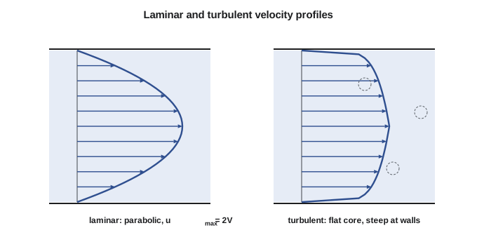
In 1883 Osborne Reynolds injected a thin stream of dye into water flowing through a glass tube. At low velocities the dye stayed in a neat straight thread: the flow was laminar, moving in smooth layers that slid past one another. As he raised the velocity, the thread began to waver, and beyond a certain point it broke up suddenly and spread through the whole tube: the flow had become turbulent, filled with irregular eddies of many sizes. Reynolds showed that the change depends not on velocity alone but on a dimensionless combination of velocity, diameter, density and viscosity, now called the Reynolds number.
The Reynolds number is the ratio of inertial forces to viscous forces. When it is small, viscosity damps out disturbances and the flow stays laminar; when it is large, disturbances grow and the flow becomes turbulent. In pipes, flow is generally laminar below \(Re \approx 2300\) and fully turbulent above about 4000, with a transitional range in between where the flow switches back and forth. Water mains run at Reynolds numbers in the hundreds of thousands to millions, so their flow is always turbulent. Laminar pipe flow occurs with viscous oils, in very small tubes and at very low velocities, such as in chemical dosing lines.
Worked problem
Reynolds numbers in the station
Find the Reynolds number for (a) water at 20 °C flowing at 1.59 m/s (5.22 ft/s) in the 600 mm (24 in) main, and (b) hypochlorite solution (\(\nu = 1.3 \times 10^{-6}\ \text{m}^2/\text{s}\)) flowing at 11 L/h (2.9 gal/h) in a 6 mm dosing tube.
Show solution
- (a) \(Re = VD/\nu = 1.59(0.600)/(1.00 \times 10^{-6}) = 954\,000\): fully turbulent.
- (b) \(Q = 11/(3.6 \times 10^6) = 3.06 \times 10^{-6}\ \text{m}^3/\text{s}\); \(A = 2.83 \times 10^{-5}\ \text{m}^2\); \(V = 0.108\ \text{m/s}\).
- \(Re = 0.108(0.006)/(1.3 \times 10^{-6}) = 500\): laminar.
Answer: The two flows in the same building differ by a factor of almost two thousand in Reynolds number and follow entirely different friction laws.
Entrance length and fully developed flow
Where a pipe leaves a tank, the velocity is nearly uniform across its entrance. The no-slip condition then slows the fluid next to the wall, and a boundary layer grows inward until it fills the pipe. Beyond that entrance length, the velocity profile stops changing along the pipe, and the flow is fully developed. For laminar flow the entrance length is about \(0.06\,Re\,D\), which can be very long; for turbulent flow it is roughly \(4.4\,Re^{1/6}D\), typically 20 to 40 diameters. The friction formulas in this lesson apply to fully developed flow. In long mains the entrance region is a small fraction of the length and is ignored, or folded into the entrance loss coefficient of Lesson 12.
The Darcy-Weisbach equation
For fully developed flow in a straight pipe of constant diameter, the head loss due to wall friction is given by the Darcy-Weisbach equation. It says that the loss is proportional to the pipe's length in diameters and to the velocity head, with a dimensionless friction factor \(f\) as the constant of proportionality. Dimensional analysis shows that \(f\) can depend only on the Reynolds number and the relative roughness \(\varepsilon/D\), the ratio of the average height of the wall's roughness elements to the diameter.
The Darcy-Weisbach equation is valid for any Newtonian fluid, laminar or turbulent, in a pipe of any material. All the difficulty lies in finding \(f\). Other formulas, notably the Hazen-Williams equation, remain popular in North American water practice because they are simple, but they are empirical, valid only for water near room temperature in turbulent flow, and less accurate for very smooth or very rough pipes. Hana uses Darcy-Weisbach for design and keeps Hazen-Williams for comparison with older records.
Laminar flow: an exact result
For fully developed laminar flow, the momentum equation and Newton's law of viscosity can be solved exactly. The result is the Hagen-Poiseuille flow: a parabolic velocity profile, with the centerline velocity twice the average, and a pressure drop proportional to the first power of the velocity. Substituting into Darcy-Weisbach gives the friction factor directly.
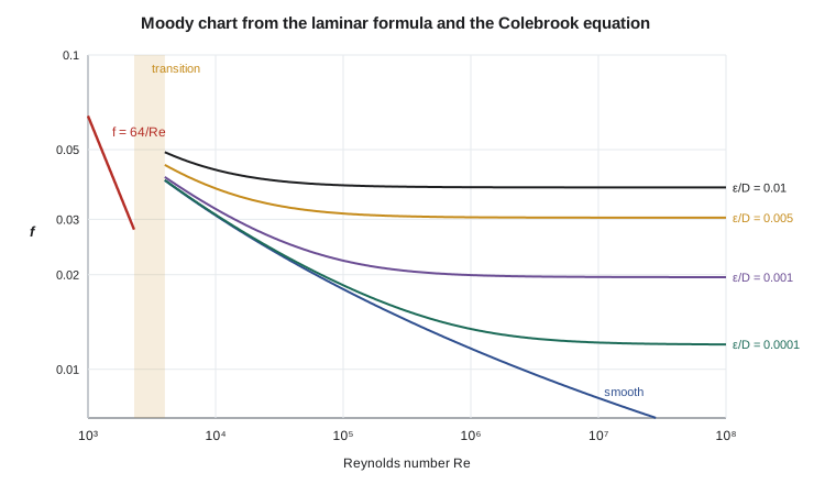
In laminar flow, wall roughness has no effect: the friction factor depends on the Reynolds number alone. Doubling the flow in a laminar dosing line doubles its pressure drop, and halving the tube diameter at the same flow multiplies the drop by sixteen. That steep dependence on diameter is why dosing tubes partly blocked by scale cause feed rates to fall sharply.
Turbulent flow and the Colebrook equation
Turbulent flow has no exact solution. Its friction factor comes from experiments, the most famous being Nikuradse's 1930s tests on pipes roughened with uniform sand grains, and from later tests on commercial pipes. In turbulent flow, a thin viscous sublayer lies next to the wall. If the roughness elements are buried inside it, the pipe behaves as hydraulically smooth and \(f\) depends only on \(Re\). If they poke through it, the pipe is rough and, at high enough Reynolds numbers, \(f\) depends only on \(\varepsilon/D\). Commercial pipes fall between these limits, and Colebrook combined the two into one implicit equation in 1939.
Because \(f\) appears on both sides, the Colebrook equation must be solved by iteration. Fortunately it converges quickly from almost any starting guess. Haaland's explicit formula, \(1/\sqrt{f} \approx -1.8\log_{10}[6.9/Re + (\varepsilon/D/3.7)^{1.11}]\), agrees within about 2 percent and makes an excellent first guess. The Moody chart, published in 1944, plots Colebrook's equation for a range of relative roughnesses and was the standard tool before computers; it remains the best way to see how friction behaves.
| Pipe material | Equivalent roughness ε (mm) | Notes |
|---|---|---|
| Drawn tubing, PVC, HDPE | 0.0015–0.007 | Hydraulically smooth in most water service |
| Commercial steel, new | 0.045 | Welded steel mains |
| Ductile iron, cement-mortar lined | 0.1–0.3 | Common for water mains |
| Cast iron, new | 0.26 | Older systems |
| Cast iron, tuberculated | 1–5 or more | Increases with age and water chemistry |
| Concrete | 0.3–3 | Depends on finish |
# Friction factor: laminar formula, Colebrook (solved by iteration) and Haaland
import math

def colebrook(Re, rel, tol=1e-12):
    if Re < 2300:
        return 64 / Re
    x = -1.8 * math.log10(6.9 / Re + (rel / 3.7) ** 1.11)   # Haaland as the starting guess, x = 1/sqrt(f)
    for _ in range(100):
        new = -2.0 * math.log10(rel / 3.7 + 2.51 * x / Re)
        if abs(new - x) < tol: break
        x = new
    return 1 / x**2

def haaland(Re, rel):
    return (-1.8 * math.log10(6.9 / Re + (rel / 3.7) ** 1.11)) ** -2

print("    Re      e/D      f Colebrook   f Haaland   diff %")
for Re in (1e3, 1e4, 1e5, 1e6, 1e7):
    for rel in (0.0, 1e-4, 1e-3, 1e-2):
        fc = colebrook(Re, rel)
        fh = haaland(Re, rel) if Re >= 2300 else fc
        print(f"{Re:8.0e}  {rel:7.4f}   {fc:10.5f}   {fh:9.5f}   {100*(fh-fc)/fc:6.2f}")

# Head loss in 1.8 km of 600 mm ductile iron main (cement lined, e = 0.25 mm assumed)
rho, mu, g = 998.0, 1.0e-3, 9.81
D, L, e, Q = 0.600, 1800.0, 0.25e-3, 0.45
V = Q / (math.pi * D**2 / 4)
Re = rho * V * D / mu
f = colebrook(Re, e / D)
hf = f * L / D * V**2 / (2 * g)
print()
print(f"Transmission main: V = {V:.2f} m/s, Re = {Re:,.0f}, f = {f:.4f}, hf = {hf:.2f} m ({rho*g*hf/1000:.0f} kPa)")Re e/D f Colebrook f Haaland diff % 1e+03 0.0000 0.06400 0.06400 0.00 1e+03 0.0001 0.06400 0.06400 0.00 1e+03 0.0010 0.06400 0.06400 0.00 1e+03 0.0100 0.06400 0.06400 0.00 1e+04 0.0000 0.03088 0.03089 0.01 1e+04 0.0001 0.03104 0.03099 -0.15 1e+04 0.0010 0.03238 0.03217 -0.64 1e+04 0.0100 0.04313 0.04304 -0.19 1e+05 0.0000 0.01799 0.01782 -0.92 1e+05 0.0001 0.01851 0.01827 -1.34 1e+05 0.0010 0.02217 0.02197 -0.94 1e+05 0.0100 0.03850 0.03854 0.09 1e+06 0.0000 0.01165 0.01159 -0.50 1e+06 0.0001 0.01344 0.01333 -0.86 1e+06 0.0010 0.01994 0.01994 -0.01 1e+06 0.0100 0.03796 0.03804 0.19 1e+07 0.0000 0.00810 0.00813 0.35 1e+07 0.0001 0.01217 0.01217 -0.00 1e+07 0.0010 0.01967 0.01970 0.18 1e+07 0.0100 0.03791 0.03799 0.20 Transmission main: V = 1.59 m/s, Re = 953,020, f = 0.0166, hf = 6.45 m (63 kPa)
Worked problem
Head loss in the transmission main
The 600 mm (24 in) cement-lined ductile iron transmission main is 1.8 km (5900 ft) long and carries 0.45 m³/s (7130 gpm) of water at 20 °C (68 °F). Taking \(\varepsilon = 0.25\ \text{mm}\), find the friction factor and the head loss, in meters and feet.
Show solution
- \(V = 0.45/0.2827 = 1.59\ \text{m/s}\); \(Re = 1.59(0.600)/10^{-6} = 9.5 \times 10^5\); \(\varepsilon/D = 0.000417\).
- Haaland first guess: \(f \approx 0.0165\). Iterating Colebrook converges to \(f = 0.0166\).
- \(h_f = 0.0166(1800/0.600)(1.59^2/19.62) = 0.0166(3000)(0.129) = 6.45\ \text{m} = 21.2\ \text{ft}\).
Answer: Friction costs 6.45 m of head, about 63 kPa, over 1.8 km. If tuberculation raised the roughness to 3 mm, the friction factor would rise to about 0.030 and the loss to about 11.8 m, an increase of more than 80 percent that the pumps would pay for every hour they run.
Using the friction factor in design
Pipe problems come in three kinds. In the first, the flow and pipe are known and the head loss is wanted, which is direct, as in the example. In the second, the head available and the pipe are known and the flow is wanted; since the friction factor depends on the unknown flow through \(Re\), we guess \(f\), compute \(V\), update \(Re\) and \(f\), and repeat until it settles. In the third, the flow and allowable loss are known and the diameter is wanted, which also needs iteration, or a sweep of standard sizes. Hana's design spreadsheets do exactly this, sweeping pipe sizes and comparing the capital cost of each with the present value of the pumping energy it requires.
Head loss in turbulent flow rises roughly with the square of velocity, more precisely with about the 1.8th to 2nd power, so a pipe carrying double its design flow loses about four times the head. Diameter matters even more. At a fixed flow, velocity varies as \(1/D^2\), so the friction loss varies roughly as \(1/D^5\): going from a 500 mm to a 600 mm main cuts friction loss by about 60 percent. That steep dependence is why small savings in pipe diameter at construction often cost far more in energy over the pipe's life.
Common mistakes
MistakeUsing f = 64/Re for turbulent flow.
Instead64/Re applies only to laminar flow (Re < 2300); use Colebrook or the Moody chart above about 4000.
MistakeConfusing the Darcy friction factor with the Fanning friction factor.
InsteadThe Fanning factor is one quarter of the Darcy factor; check which one a chart or formula uses.
MistakeUsing relative roughness in millimeters.
Insteadε/D is dimensionless; use the same units for ε and D.
MistakeAssuming smooth plastic pipe has zero friction.
InsteadEven smooth pipes have f ≈ 0.01–0.02 in turbulent flow.
MistakeApplying Hazen-Williams to oil or laminar flow.
InsteadIt is empirical, for water in turbulent flow; use Darcy-Weisbach for other cases.
Summary and key terms
- The Reynolds number Re = ρVD/μ separates laminar (Re < 2300) from turbulent (Re > 4000) pipe flow.
- Darcy-Weisbach: h_f = f(L/D)(V²/2g) for any fluid and flow regime.
- Laminar flow has a parabolic profile and f = 64/Re, independent of roughness.
- Turbulent f depends on Re and ε/D and is found from the Colebrook equation, the Haaland formula or the Moody chart.
- At high Re in rough pipes, f becomes constant (fully rough flow).
- Friction loss rises with roughly V² and falls with roughly D⁻⁵ at fixed flow.
- Reynolds number
- The ratio of inertial to viscous forces, Re = ρVD/μ.
- Laminar flow
- Smooth, layered flow in which viscosity damps out disturbances.
- Turbulent flow
- Flow filled with irregular eddies that mix fluid across the pipe.
- Entrance length
- The distance from a pipe inlet to where the velocity profile becomes fully developed.
- Fully developed flow
- Flow whose velocity profile does not change along the pipe.
- Darcy-Weisbach equation
- h_f = f(L/D)V²/(2g), the general law for friction loss in pipes.
- Friction factor
- The dimensionless factor f in the Darcy-Weisbach equation.
- Relative roughness
- Equivalent wall roughness divided by diameter, ε/D.
- Colebrook equation
- The implicit relation for the turbulent friction factor in commercial pipes.
- Moody chart
- A plot of friction factor against Reynolds number for various relative roughnesses.
- Viscous sublayer
- The thin layer next to the wall in turbulent flow where viscous effects dominate.
Practice problems
Work each problem on paper first, then reveal the answer to check.
Oil with ν = 5 × 10⁻⁵ m²/s flows at 0.8 m/s in a 50 mm pipe. Is the flow laminar? Find f.
Show answer
Re = 800, laminar; f = 64/800 = 0.08.
Find the head loss for that oil in 30 m of the pipe.
Show answer
h_f = 0.08(30/0.05)(0.8²/19.62) = 1.57 m.
Water at 20 °C flows at 2 m/s in a 200 mm PVC pipe (ε ≈ 0.0015 mm). Find Re and f.
Show answer
Re = 4.0 × 10⁵; f ≈ 0.0138 (nearly smooth).
A pipe's flow doubles in fully rough turbulent flow. By what factor does the head loss change?
Show answer
About 4, since f is constant and h_f ∝ V².
Estimate how much a 600 mm main reduces friction loss compared with a 500 mm main at the same flow.
Show answer
About (500/600)⁵ = 0.40, so a 60 % reduction.
In the program, change the main's roughness to 3 mm. What are the new f and h_f?
Show answer
f ≈ 0.030 and h_f ≈ 11.8 m.
Lesson quiz · 5 questions
Score 60% or more to complete this lesson.
Create a free account to save your progress, take quizzes and earn a certificate.