
CIV-241 · Lesson 8 of 12 · 22 min
Groundwater and Darcy's law
Water is involved in most geotechnical problems. It reduces effective stress and therefore strength, drives landslides, floods excavations, causes piping beneath dams, carries contaminants, supplies drinking water and, when pumped out, makes the ground settle. Hydrogeology, the study of groundwater, is a large field of its own, but every civil engineer needs the basic ideas: where groundwater occurs, how it moves, and how to estimate flow rates with Darcy's law. This lesson builds that foundation, using Kestrel's reservoir and well field project as the running example.
The hydrologic cycle and where groundwater occurs
Precipitation that falls on land either runs off, evaporates, is taken up by plants, or infiltrates into the ground. Infiltrating water first passes through the unsaturated (vadose) zone, where pores contain both air and water, and then reaches the saturated zone, where all pores are filled with water. The top of the saturated zone is the water table, where the pore water pressure equals atmospheric pressure. Just above the water table, capillary forces hold water in a capillary fringe that may be centimeters thick in gravel and meters thick in fine silts and clays.
Groundwater moves slowly through the saturated zone from recharge areas, usually uplands, toward discharge areas such as springs, rivers, lakes, wetlands and wells. The water table generally follows the shape of the ground surface in a subdued way, higher beneath hills and lower beneath valleys, and it rises and falls seasonally. In much of Canada and the northern United States, water tables are highest in spring after snowmelt and lowest in late summer or winter, which is why landslides and excavation problems often peak in spring.
Aquifers and aquitards
An aquifer is a geologic unit that can store and transmit enough water to supply wells or springs. Good aquifers include clean sand and gravel, such as glacial outwash and eskers, porous sandstone, fractured or karstic limestone, and fractured or rubbly zones in volcanic rocks. An aquitard is a unit of low permeability, such as clay, till, shale or unfractured crystalline rock, that slows but does not entirely stop water movement. An aquiclude is an essentially impermeable unit, a term now used less often because few units are truly impermeable over long times.
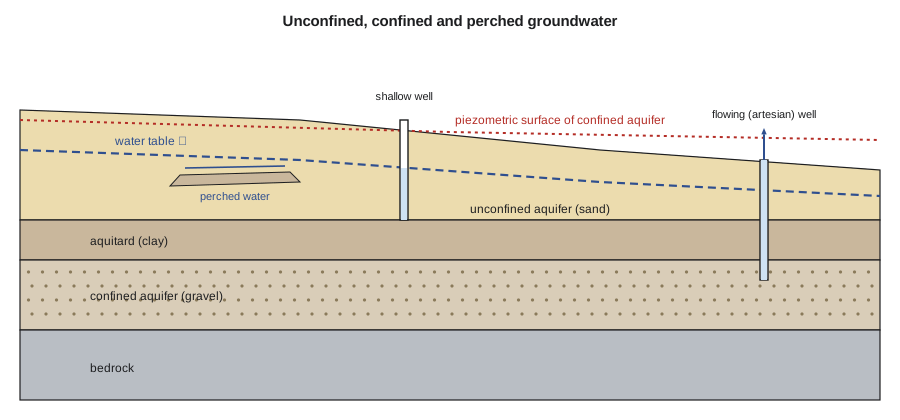
An unconfined aquifer has the water table as its upper boundary and is recharged directly from above. A confined aquifer lies between aquitards and holds water under pressure. If a well is drilled into a confined aquifer, water rises in it above the top of the aquifer to a level called the piezometric (potentiometric) surface. If that surface is above the ground, the well flows without pumping, an artesian condition. A perched water table forms where a local lens of low-permeability material, such as a clay layer within sand, holds up a small saturated zone above the main water table. Perched water often surprises contractors because it appears in excavations well above the regional water table shown in reports.
Hydraulic head
Groundwater flows from points of high total hydraulic head to points of low total head, not necessarily from high pressure to low pressure or from high elevation to low elevation. The total head at a point is the sum of the elevation head, the height of the point above a chosen datum, and the pressure head, the pore water pressure divided by the unit weight of water. Velocity head is negligible in groundwater because flow is so slow.
In practice, total head is measured with a piezometer: a pipe or sensor sealed at a particular depth, which records the water pressure there. The level to which water rises in an open standpipe piezometer is the total head at its tip. Several piezometers at different depths in the same location show whether flow is downward (head decreasing with depth, typical of recharge areas) or upward (head increasing with depth, typical of discharge areas, and a concern beneath excavations where it can cause heave or boiling).
Darcy's law
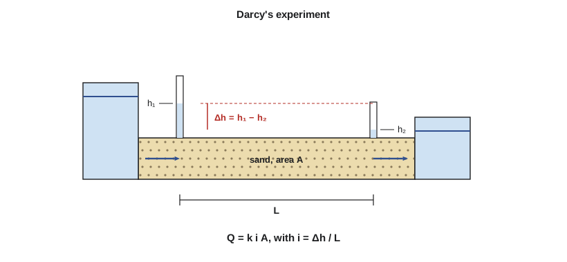
In 1856, the French engineer Henry Darcy, designing sand filters for the water supply of Dijon, showed experimentally that the rate of water flow through a column of sand is proportional to the head loss and the cross-sectional area and inversely proportional to the length of the column. In modern form, Darcy's law is:
Here \(Q\) is the flow rate (m³/s), \(k\) the hydraulic conductivity (m/s), \(i\) the hydraulic gradient (head loss per unit length, dimensionless), \(A\) the total cross-sectional area perpendicular to flow, and \(v\) the Darcy velocity or specific discharge. Because water flows only through the pores, the actual average speed of water particles, the seepage velocity, is faster: \(v_s = v / n_e\), where \(n_e\) is the effective porosity. The seepage velocity is what matters for estimating how quickly a contaminant or tracer moves.
Darcy's law applies to laminar flow, which covers nearly all groundwater flow in soils. It can break down in very coarse gravel, in large open fractures and karst conduits, and near pumping wells in coarse material, where flow becomes turbulent.
Hydraulic conductivity
Hydraulic conductivity, often loosely called permeability, varies over more than ten orders of magnitude among natural materials, far more than almost any other engineering property. That range is why rough estimates are often adequate for deciding whether a material is a drain or a barrier, while design of dewatering or water supply needs field testing.
| Material | Typical hydraulic conductivity k (m/s) | Behavior |
|---|---|---|
| Clean gravel | 10⁻³ to 10⁻¹ | Very permeable; excellent aquifer; large inflows |
| Clean sand, sand and gravel | 10⁻⁵ to 10⁻² | Good aquifer; drains freely |
| Silty sand, fine sand | 10⁻⁷ to 10⁻⁵ | Moderate to low |
| Silt, loess | 10⁻⁹ to 10⁻⁶ | Low; slow drainage |
| Glacial till | 10⁻¹² to 10⁻⁶ | Low; depends on matrix and fractures |
| Clay (unfractured) | 10⁻¹³ to 10⁻⁹ | Practically impermeable over short times |
| Fractured or karstic rock | 10⁻⁸ to 10⁻² | Controlled by fractures and conduits |
| Unfractured crystalline rock | 10⁻¹⁴ to 10⁻¹⁰ | Very low |
For clean, uniform sands, Hazen's empirical formula gives a rough estimate from the effective size \(D_{10}\): \(k \approx C D_{10}^2\), with \(k\) in cm/s, \(D_{10}\) in mm and \(C\) about 1 (with a range of roughly 0.4 to 1.5). It does not work for silty or clayey soils or for well-graded materials. In layered deposits such as varved clays and alluvium, the horizontal conductivity can be ten to a hundred times the vertical, because water flows easily along permeable layers but must cross the least permeable layers to move vertically.
Field tests measure conductivity at the scale that matters. Rising- and falling-head tests in boreholes or piezometers test a small volume of ground around the screen. Packer tests isolate sections of a borehole in rock. Pumping tests, in which a well is pumped at a steady rate while drawdown is measured in nearby observation wells, test a large volume of aquifer and are the standard for water supply and major dewatering design.
Worked problem
Seepage through a layered deposit and flow to a well
(a) At the reservoir site, a 6.0 m (19.7 ft) thick deposit consists of 4.0 m of sand with \(k = 2 \times 10^{-4}\) m/s and 2.0 m of silt with \(k = 1 \times 10^{-7}\) m/s. Find the equivalent horizontal and vertical conductivities. (b) A production well fully penetrates a confined gravel aquifer 12 m (39 ft) thick with \(k = 8 \times 10^{-4}\) m/s. At steady pumping, observation wells 10 m and 60 m away show drawdowns of 3.2 m and 1.1 m. Estimate the pumping rate using the Thiem equation, and express it in US gallons per minute.
Show solution
- (a) Horizontal conductivity is the thickness-weighted average:
- \[k_h = \frac{4.0(2 \times 10^{-4}) + 2.0(1 \times 10^{-7})}{6.0} = 1.33 \times 10^{-4}\ \text{m/s}\]
- Vertical conductivity is governed by the least permeable layer:
- \[k_v = \frac{6.0}{4.0/(2 \times 10^{-4}) + 2.0/(1 \times 10^{-7})} = \frac{6.0}{20\,000 + 20\,000\,000} = 3.0 \times 10^{-7}\ \text{m/s}\]
- (b) For steady radial flow in a confined aquifer of thickness \(b\), the Thiem equation is:
- \[Q = \frac{2 \pi k b\, (s_1 - s_2)}{\ln(r_2 / r_1)} = \frac{2\pi (8 \times 10^{-4})(12)(3.2 - 1.1)}{\ln(60/10)}\]
- \[Q = \frac{0.1267}{1.792} = 0.0707\ \text{m}^3/\text{s} \approx 71\ \text{L/s}\]
- Converting, 1 L/s is about 15.85 US gal/min:
- \[Q \approx 71 \times 15.85 \approx 1120\ \text{gal/min}\]
Answer: (a) \(k_h \approx 1.3 \times 10^{-4}\) m/s and \(k_v \approx 3 \times 10^{-7}\) m/s, a ratio of more than 400: the silt layer controls vertical flow. (b) The well is pumping about 71 L/s, or roughly 1,100 US gal/min.
# Darcy flow, seepage velocity, layered conductivity and Thiem well flow
import math

# Seepage through a sand layer beneath a cofferdam
k, dh, L, A, ne = 2e-4, 3.0, 15.0, 40.0, 0.30
i = dh / L
Q = k * i * A
v = Q / A
print(f"gradient i = {i:.2f}, Q = {Q*1000:.2f} L/s, Darcy v = {v:.2e} m/s, seepage v = {v/ne:.2e} m/s")
print(f"travel time across {L} m: {L/(v/ne)/86400:.1f} days")

# Equivalent conductivity of layers (thickness m, k m/s)
layers = [(4.0, 2e-4), (2.0, 1e-7)]
H = sum(d for d, _ in layers)
kh = sum(d * kk for d, kk in layers) / H
kv = H / sum(d / kk for d, kk in layers)
print(f"kh = {kh:.2e} m/s, kv = {kv:.2e} m/s, kh/kv = {kh/kv:.0f}")

# Thiem equation for a confined aquifer
kq, b, r1, s1, r2, s2 = 8e-4, 12.0, 10.0, 3.2, 60.0, 1.1
Qw = 2 * math.pi * kq * b * (s1 - s2) / math.log(r2 / r1)
print(f"well yield = {Qw*1000:.0f} L/s")

# Hazen estimate for clean sand
for d10 in (0.1, 0.25, 0.5):
print(f"D10 = {d10} mm -> k ~ {1.0 * d10**2 / 100:.1e} m/s")gradient i = 0.20, Q = 1.60 L/s, Darcy v = 4.00e-05 m/s, seepage v = 1.33e-04 m/s travel time across 15.0 m: 1.3 days kh = 1.33e-04 m/s, kv = 3.00e-07 m/s, kh/kv = 445 well yield = 71 L/s D10 = 0.1 mm -> k ~ 1.0e-04 m/s D10 = 0.25 mm -> k ~ 6.3e-04 m/s D10 = 0.5 mm -> k ~ 2.5e-03 m/s
Groundwater and engineering problems
Groundwater appears in almost every lesson of this course because it affects nearly every geotechnical problem.
- Effective stress and strength: the strength of soil and of discontinuities in rock depends on effective stress, the total stress minus pore water pressure. Raising the water table or the water pressure on a joint reduces effective stress and strength, which is why landslides are often triggered by rainfall and snowmelt.
- Excavations and dewatering: excavations below the water table in permeable soils need dewatering by sumps, well points or deep wells, or cut-off walls. Upward gradients beneath an excavation base can cause boiling and heave if the effective stress falls to zero; the critical gradient is about 1.0 for typical soils.
- Piping and internal erosion: water flowing through soil at high gradients can carry fine particles away, forming pipes that grow and can lead to dam and levee failures. Filters graded to hold the soil while passing water are the standard defense.
- Settlement from pumping: lowering the water table increases effective stress in compressible layers and causes settlement, sometimes damaging nearby buildings and utilities.
- Water supply and contamination: wells, springs and municipal well fields must be protected from contamination, and construction near them must avoid introducing pollutants or altering flow paths.
In the United States, groundwater rights and protection are governed mainly by state law, which varies widely, from prior appropriation in most western states to reasonable use doctrines in many eastern states. Washington requires water right permits for most non-domestic groundwater withdrawals, with an exemption for small domestic and stock wells, and the state Department of Ecology maintains well log records. Kestrel's well field design for the reservoir must therefore include a water right application, and the firm uses state well logs to understand the aquifer before drilling test wells.
Common mistakes
MistakeAssuming water flows from high pressure to low pressure.
InsteadWater flows from high to low total head, the sum of elevation and pressure heads.
MistakeUsing the Darcy velocity to estimate contaminant travel time.
InsteadUse the seepage velocity, the Darcy velocity divided by effective porosity, which is faster.
MistakeAveraging conductivities of layers arithmetically for vertical flow.
InsteadVertical flow is controlled by the least permeable layers; use the harmonic (series) formula.
MistakeRelying on a single water level reading from a borehole.
InsteadWater levels vary seasonally and may not have stabilized; install piezometers and monitor over time.
Summary and key terms
- Groundwater fills the saturated zone below the water table and moves from recharge to discharge areas.
- Aquifers transmit water readily; aquitards slow it; confined aquifers are pressurized and can produce artesian flow.
- Flow is driven by differences in total head \(h = z + u/\gamma_w\), measured with piezometers.
- Darcy's law: \(Q = kiA\); seepage velocity is \(v/n_e\).
- Hydraulic conductivity spans more than ten orders of magnitude; layered deposits have \(k_h\) much greater than \(k_v\).
- Groundwater controls effective stress, excavation stability, piping, settlement from pumping and water supply.
- Water table
- The surface in the ground where pore water pressure equals atmospheric pressure.
- Aquifer
- A geologic unit that stores and transmits water in useful quantities.
- Aquitard
- A low-permeability unit that slows groundwater movement.
- Confined aquifer
- An aquifer bounded above and below by aquitards and holding water under pressure.
- Hydraulic head
- The sum of elevation head and pressure head; groundwater flows from high to low head.
- Hydraulic conductivity
- The coefficient in Darcy’s law relating flow velocity to hydraulic gradient.
- Seepage velocity
- The average speed of water through the pores, equal to the Darcy velocity divided by effective porosity.
- Piezometer
- An instrument that measures pore water pressure or head at a point.
Practice problems
Work each problem on paper first, then reveal the answer to check.
A sand sample 0.30 m long with area 0.01 m² passes 1.5 × 10⁻⁵ m³/s under a head loss of 0.45 m. What is k?
Show answer
\(i = 1.5\), so \(k = Q/(iA) = 1.5\times10^{-5}/(1.5 \times 0.01) = 1.0 \times 10^{-3}\) m/s.
What is a perched water table?
Show answer
A local saturated zone held up by a low-permeability lens above the main water table.
Why is the seepage velocity greater than the Darcy velocity?
Show answer
Water flows only through the pore space, which is a fraction of the total area.
Estimate k for a clean sand with \(D_{10} = 0.2\) mm using Hazen's formula.
Show answer
\(k \approx 0.2^2 = 0.04\) cm/s \(= 4 \times 10^{-4}\) m/s.
Why can upward seepage beneath an excavation be dangerous?
Show answer
It reduces effective stress; at the critical gradient the soil boils and loses strength.
What field test best measures aquifer conductivity at large scale?
Show answer
A pumping test with observation wells.
Lesson quiz · 5 questions
Score 60% or more to complete this lesson.
Create a free account to save your progress, take quizzes and earn a certificate.