
CHE-374 · Lesson 6 of 12 · 22 min
Feedback control and the PID controller
With a model of tray 13 in hand, Theo turns to the controller. Almost every loop at Kingfisher Bioenergy, several hundred of them, uses the same algorithm: proportional-integral-derivative, or PID, in one of its forms. It has survived nearly a century of competition from cleverer methods because it is simple, robust and understood by operators. Using it well depends on details that textbooks often skip: which way it acts, which form the vendor implemented, how derivative is filtered, and what the valve in the field actually does with the signal.
Proportional action
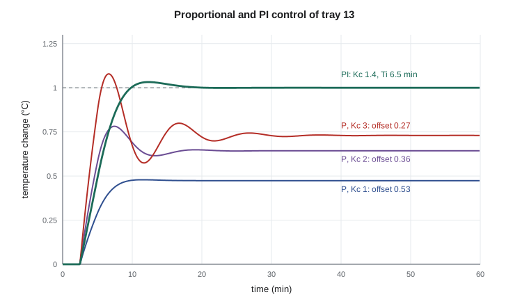
Proportional action makes the controller output change in proportion to the error, \(u = \bar u + K_c e\), where \(e = y_{sp} - y\) and \(\bar u\) is the bias, the output at zero error. Many DCS vendors express the gain as a proportional band, the percentage change in measurement that drives the output across its full range: \(PB = 100/K_c\) when both are in percent of span. A small band means a high gain. Lesson 1 showed the drawback of proportional action alone: after a sustained load change it leaves an offset. For the tray temperature, with \(K = 0.90\) °C per percent, a set-point step of 1 °C settles with an offset of \(1/(1 + K K_c)\): 0.53 °C at \(K_c = 1\), 0.36 °C at 2 and 0.27 °C at 3 %/°C. Raising the gain reduces the offset but makes the response oscillate: at \(K_c = 3\) the temperature overshoots its final value by almost 50 % and swings for several cycles. Proportional-only control is still used where offset does not matter, such as averaging level control in lesson 12.
# Feedback control of the tray temperature (FOPDT from lesson 5) and installed valve gain
import math, random
def fopdt_step(K, tau, theta, t):
    # response of K e^(-theta s)/(tau s + 1) to a unit step at t = 0
    return 0.0 if t < theta else K * (1 - math.exp(-(t - theta) / tau))
class Plant:
    # first- or second-order lag with dead time, stepped with Euler at a small dt
    def __init__(self, K, tau1, theta, dt, tau2=0.0):
        self.K, self.t1, self.t2, self.dt = K, tau1, tau2, dt
        self.buf = [0.0] * max(1, int(round(theta / dt)))
        self.x1 = 0.0; self.x2 = 0.0
    def step(self, u):
        self.buf.append(u); ud = self.buf.pop(0)
        self.x1 += self.dt * (self.K * ud - self.x1) / self.t1
        if self.t2 > 0:
            self.x2 += self.dt * (self.x1 - self.x2) / self.t2
            return self.x2
        return self.x1
def loop(K, tau, theta, Kc, Ti, Td=0.0, tend=60.0, dt=0.01, sp=1.0, load=0.0, t_load=0.0,
         umin=-1e9, umax=1e9, antiwindup=True, tau2=0.0):
    # PI(D) control of an FOPDT (or SOPDT) plant; derivative acts on the measurement.
    # A load enters at the plant input at t_load. Returns lists of t, y, u.
    p = Plant(K, tau, theta, dt, tau2)
    I, ylast, y = 0.0, 0.0, 0.0
    T, Y, U = [], [], []
    n = int(tend / dt)
    for k in range(n):
        t = k * dt
        e = sp - y
        D = -Kc * Td * (y - ylast) / dt if Td > 0 else 0.0
        u_un = Kc * e + I + D
        u = min(umax, max(umin, u_un))
        if Ti > 0:
            if not antiwindup or u == u_un or (u_un > umax and e < 0) or (u_un < umin and e > 0):
                I += Kc * dt / Ti * e
        d = load if t >= t_load else 0.0
        ylast = y
        y = p.step(u + d)
        T.append(t); Y.append(y); U.append(u)
    return T, Y, U
def iae(T, Y, sp, t0=0.0):
    dt = T[1] - T[0]
    return sum(abs(sp - y) * dt for t, y in zip(T, Y) if t >= t0)
def overshoot(Y, sp):
    return max(0.0, (max(Y) - sp) / sp * 100) if sp else 0.0
def settle(T, Y, sp, band=0.05):
    last = T[0]
    for t, y in zip(T, Y):
        if abs(y - sp) > band * abs(sp): last = t
    return last
K, tau, theta = 0.90, 6.5, 2.5             # degC per % steam, min, min
print("Setpoint +1 degC on the tray temperature:")
for Kc in (1.0, 2.0, 3.0):
    T, Y, U = loop(K, tau, theta, Kc, 0.0, tend=120)
    print(f"  P only, Kc = {Kc:.1f} %/degC: final {Y[-1]:.3f} degC, offset {1 - Y[-1]:.3f} (theory 1/(1+K Kc) = {1 / (1 + K * Kc):.3f}), peak {max(Y):.3f}")
T, Y, U = loop(K, tau, theta, 1.4, 6.5, tend=120)
print(f"  PI, Kc = 1.4, Ti = 6.5 min: final {Y[-1]:.3f} degC, overshoot {overshoot(Y, 1):.1f} %, settles (5 %) at {settle(T, Y, 1):.1f} min")
T, Y, U = loop(K, tau, theta, 1.4, 6.5, tend=120, sp=0.0, load=-2.0, t_load=0.0)
last = max(t for t, y in zip(T, Y) if abs(y) > 0.05)
print(f"  PI rejecting a -2 % steam load: worst deviation {min(Y):.3f} degC, back within 0.05 degC after {last:.1f} min")
# Installed characteristics: flow fraction q at valve lift l, with authority N = valve share of the pressure drop at full flow
import math
R, N = 50.0, 0.10
def phi(l, kind): return l if kind == 'linear' else R ** (l - 1)
def q(l, kind): return 1 / math.sqrt((1 - N) + N / phi(l, kind) ** 2)
print("lift   linear valve: q  gain dq/dl   equal-%: q  gain dq/dl")
for l in (0.2, 0.5, 0.8):
    g = [(q(l + 0.01, k) - q(l - 0.01, k)) / 0.02 for k in ('linear', 'eqp')]
print(f" {l:.1f} {q(l, 'linear'):.3f} {g[0]:.2f} {q(l, 'eqp'):.3f} {g[1]:.2f}")Setpoint +1 degC on the tray temperature: P only, Kc = 1.0 %/degC: final 0.474 degC, offset 0.526 (theory 1/(1+K Kc) = 0.526), peak 0.479 P only, Kc = 2.0 %/degC: final 0.643 degC, offset 0.357 (theory 1/(1+K Kc) = 0.357), peak 0.781 P only, Kc = 3.0 %/degC: final 0.730 degC, offset 0.270 (theory 1/(1+K Kc) = 0.270), peak 1.077 PI, Kc = 1.4, Ti = 6.5 min: final 1.000 degC, overshoot 3.2 %, settles (5 %) at 8.7 min PI rejecting a -2 % steam load: worst deviation -0.821 degC, back within 0.05 degC after 26.7 min lift linear valve: q gain dq/dl equal-%: q gain dq/dl 0.2 0.542 1.99 0.137 0.53 0.5 0.877 0.54 0.412 1.36 0.8 0.973 0.18 0.852 1.16
Integral action
Integral action adds a term proportional to the accumulated error:
As long as any error remains, the integral keeps changing the output, so the only possible steady state is zero error. The integral time \(T_i\), in minutes, is the time the integral term takes to repeat the proportional action for a constant error; some systems use its inverse, repeats per minute. With \(K_c = 1.4\) %/°C and \(T_i = 6.5\) min, the tray loop reaches its new set point with about 3 % overshoot and settles within 9 minutes. Against a load, a 2 % drop in effective steam caused by a header pressure dip, the temperature falls at most 0.82 °C and returns within 0.05 °C in about 27 minutes. Integral action brings two costs: it adds phase lag, which makes the loop more prone to oscillate, and it winds up when the output saturates, a problem treated in lesson 8.
Derivative action
Derivative action adds a term proportional to the rate of change of the error, \(K_c T_d\, de/dt\). It anticipates where the error is heading and can let a loop with lag-dominant dynamics run faster. It also amplifies measurement noise, so in practice it is applied with a filter, typically with a time constant one-tenth to one-twentieth of \(T_d\), and it is applied to the measurement rather than to the error. Acting on the measurement avoids a large kick in the output, called derivative kick, every time the operator changes the set point. On flow and pressure loops, which are fast and noisy, derivative is almost never used. On temperature loops with large thermal lags it can help. On composition loops with analyzer dead time it rarely does, because no amount of anticipation can see through a dead time.
Forms of the PID algorithm
Vendors implement PID in different forms, and settings copied between them without conversion give different behavior. The ideal, or parallel-interacting, form multiplies all three terms by \(K_c\): \(K_c[1 + 1/(T_i s) + T_d s]\). The series form, used by many older analog controllers and still offered by some systems, is \(K_c'(1 + 1/(T_i' s))(1 + T_d' s)\). Expanding the series form shows that its effective gain is \(K_c'(1 + T_d'/T_i')\). When derivative is not used the two forms are identical, which is one reason PI controllers travel well between systems. Malik's rule is that tuning values are always recorded with the form, units and vendor they belong to.
| Setting | Typical name in a DCS | Units | Effect of increasing it |
|---|---|---|---|
| Proportional gain | gain or proportional band | % output per % measurement | Faster, more oscillatory; band moves the opposite way |
| Integral time | reset or integral time | minutes (or repeats per minute) | Slower integral action; more stable, slower to remove offset |
| Derivative time | rate or derivative time | minutes | More anticipation and more noise amplification |
Direct and reverse action
A controller must push the manipulated variable in the direction that corrects the error. When the tray temperature is too high, the steam should fall. Since more steam raises the temperature, the process gain is positive, and the controller must be reverse acting: its output falls when the measurement rises. The reflux drum level controller of lesson 1 is the opposite: a high level must open the outflow valve, so it is direct acting. Getting the action wrong makes a negative feedback loop into a positive one, and the loop drives itself to a limit within a few time constants. It is one of the most common commissioning errors, and in the wrong place it is dangerous.
Worked problem
Choosing the action
A cooling-water valve on the decanter's condenser controls the decanter temperature. The valve is fail-open, so a rising signal closes it. Should the temperature controller be direct or reverse acting?
Show solution
- If the temperature rises, more cooling is needed, so the valve must open.
- Opening this valve requires a falling signal, because it is fail-open.
- So a rising temperature must give a falling output: reverse acting.
Answer: Reverse acting. With an air-to-open valve the same loop would need direct action.
The final control element
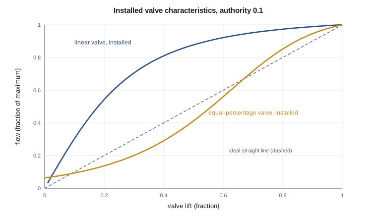
The controller's output means nothing until a valve moves. Control valves are chosen to fail to a safe position on loss of air or signal: the reboiler steam valve fails closed, the decanter cooling-water valve fails open. Their inherent characteristic, the relationship between stem travel and flow at constant pressure drop, is usually linear or equal percentage. In service, the pressure drop across the valve falls as it opens and the line losses grow, so the installed characteristic differs from the inherent one. The authority \(N\), the valve's share of the system pressure drop at full flow, decides how much. With \(N = 0.10\), the code shows that a linear valve's installed gain falls from about 2.0 at 20 % lift to 0.2 at 80 %, a tenfold change, while an equal-percentage valve with rangeability 50 varies only between about 0.5 and 1.4. Because loop gain is the product of controller, valve and process gains, an equal-percentage valve in a system with low authority keeps the loop's behavior much more uniform across its range.
Valve problems cause more poor loop performance than poor tuning. Stiction makes the valve stick and then jump, producing a characteristic sawtooth limit cycle that no tuning can remove. Hysteresis and deadband mean small output changes do nothing. An oversized valve operates near its seat, where its gain is high and its resolution poor. Malik's first check on any misbehaving loop is to put it in manual and make small output steps, 0.5 % at a time, to see whether the valve actually moves.
Putting the loop together
The closed-loop transfer function from set point to measurement, using the block-diagram rule of lesson 3, is \(G_cG_vG_pG_m/(1 + G_cG_vG_pG_m)\). The product in the denominator, the loop gain, includes the transmitter span and the valve characteristic as well as the process. Changing a transmitter's range from 0 to 150 °C to 50 to 100 °C triples the loop gain in percent terms, and the loop may start oscillating with the same tuning. Theo learns to keep a loop sheet with every element's span and characteristic, so that a tuning that worked can be explained.
Before any tuning, Theo checks the tray 13 loop against Malik's list. The controller is reverse acting and its output drives the steam flow, not the valve directly. The temperature transmitter's span is 70 to 110 °C. The steam valve strokes cleanly in 0.5 % steps. The DCS filter on the measurement is 3 seconds, negligible against the dead time. Only then does he move on to choosing \(K_c\) and \(T_i\), which is the subject of lessons 7 and 8.
Common mistakes
MistakeCopying PID settings between vendors without checking the form.
InsteadIdeal and series forms differ when derivative is used; record the form and units.
MistakeUsing derivative on a noisy flow loop.
InsteadFast noisy loops do better with PI; filter derivative when it is used.
MistakeSetting the controller action without checking the valve's fail position.
InsteadWork through the signs: process gain, valve action and controller action.
MistakeRetuning a loop that has a sticking valve.
InsteadTest the valve in manual first; tuning cannot fix stiction.
Summary and key terms
- PID combines proportional, integral and derivative action on the error.
- Proportional control leaves an offset \(1/(1 + K K_c)\); integral action removes it.
- Derivative should act on the measurement and be filtered; it is rarely useful on noisy or dead-time-dominant loops.
- Controller action must be chosen from the signs of the process gain and the valve.
- Installed valve characteristics and transmitter spans are part of the loop gain.
- PID controller
- A controller combining proportional, integral and derivative action.
- Proportional band
- The percentage change in measurement that moves the output across its full range.
- Integral time
- The time for integral action to repeat the proportional action for a constant error.
- Derivative kick
- A spike in output caused by derivative action on a set-point step.
- Reverse acting
- A controller whose output falls when the measurement rises.
- Installed characteristic
- The relationship between valve travel and flow in the actual piping system.
- Valve authority
- The fraction of the system pressure drop taken by the valve at full flow.
Practice problems
Work each problem on paper first, then reveal the answer to check.
A proportional band of 50 % corresponds to what gain?
Show answer
\(K_c = 100/50 = 2\).
Find the offset for \(K = 0.9\) and \(K_c = 4\) after a unit set-point step.
Show answer
\(1/(1 + 3.6) = 0.22\).
A series PID has \(K_c' = 2\), \(T_i' = 8\), \(T_d' = 2\) min. What is its effective ideal-form gain?
Show answer
\(2(1 + 2/8) = 2.5\).
A reboiler steam valve fails closed. Is the tray temperature controller direct or reverse acting?
Show answer
Reverse acting: a rising temperature must reduce the signal and close the valve.
Why can a transmitter re-range make a loop oscillate?
Show answer
It changes the loop gain in percent terms.
What pattern suggests valve stiction?
Show answer
A sawtooth or square-wave limit cycle in output and measurement.
Lesson quiz · 5 questions
Score 60% or more to complete this lesson.
Create a free account to save your progress, take quizzes and earn a certificate.