Dynamic models of process units

Malik's first assignment for Theo is to understand why the decanter-water surge tank behind the ester column seems sluggish at low level and nervous at high level. The tank drains by gravity through a fixed restriction to the stripper of CHE-350, so its outflow depends on the level. Theo has spent four years writing steady-state balances. Now he needs the same balances with an accumulation term, because control is about how a process moves from one state to another and how fast.

Balances with accumulation

Every dynamic model in chemical engineering starts from the same statement: accumulation equals in minus out plus generation. Applied to total mass, a component or energy over a control volume, it gives ordinary differential equations in time when the contents are well mixed, and partial differential equations when properties vary in space, as along a pipe or a packed bed. For control work, lumped models with a few well-mixed volumes usually capture the behavior that matters. The skill is choosing what to include. A model for tuning a level loop needs the tank area and the outflow law; it does not need the temperature profile of the liquid.

For a liquid tank of constant cross-section \(A\) and constant density, the mass balance reduces to a volume balance:

If the outflow is set by a pump and control valve, \(q_{out}\) does not depend on \(h\), and the tank is a pure integrator, as the reflux drum of lesson 1 was. If the tank drains by gravity through a restriction, the flow through the restriction follows an orifice law, \(q_{out} = C_v\sqrt{h}\), and the tank regulates itself: a higher level pushes out more liquid until outflow again matches inflow.

The surge tank and linearization

The surge tank has \(A = 3.0\) m² and runs at \(h_0 = 1.5\) m with 12.0 m³/h passing through, so \(C_v = 12.0/\sqrt{1.5} = 9.80\) in units of m³/h per square root of meter. The square root makes the model nonlinear. Control theory, and the transfer functions of lesson 3, need linear models, so engineers linearize about the operating point with a first-order Taylor series. Writing deviation variables \(h' = h - h_0\) and \(q' = q_{in} - q_0\):

with \(\tau = 2A\sqrt{h_0}/C_v\) and \(K = 2\sqrt{h_0}/C_v\). At the operating point the slope of the outflow law is 4.0 (m³/h)/m, so \(\tau = 3.0/4.0 = 0.75\) h, or 45 minutes, and \(K = 0.25\) m per m³/h. That is a first-order process: a gain and a time constant. The gain says how far the level will move for a sustained change in inflow; the time constant says how long it takes to get most of the way there.

# Dynamic models: a gravity-drained surge tank (nonlinear) and a heated hold tank (linear)
import math
A, h0, q0 = 3.0, 1.5, 12.0            # m2, m, m3/h at the steady state
Cv = q0 / math.sqrt(h0)              # outflow q = Cv * sqrt(h)
slope = Cv / (2 * math.sqrt(h0))     # dq/dh at the steady state
tau, K = A / slope, 1 / slope        # linear model: tau dh'/dt = K q_in' - h'
print(f"Cv = {Cv:.3f}; dq/dh = {slope:.2f} (m3/h)/m; tau = {tau:.2f} h = {tau * 60:.0f} min; gain = {K:.3f} m per m3/h")
def rk4(f, y, h):
    k1 = f(y); k2 = f(y + h / 2 * k1); k3 = f(y + h / 2 * k2); k4 = f(y + h * k3)
    return y + h / 6 * (k1 + 2 * k2 + 2 * k3 + k4)
for pct in (10, 50):
    qin = q0 * (1 + pct / 100)
    hn = h0; hl = 0.0; dt = 0.01                 # hours
    for _ in range(int(6 / dt)):                 # six hours, about eight time constants
        hn = rk4(lambda h: (qin - Cv * math.sqrt(max(h, 0))) / A, hn, dt)
        hl = rk4(lambda x: (K * (qin - q0) - x) / tau, hl, dt)
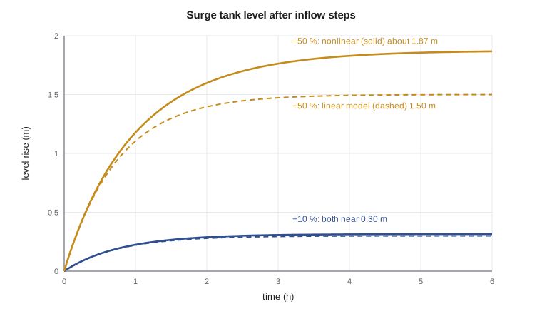
    print(f"inflow +{pct:2d} %: nonlinear level rise {hn - h0:.3f} m, linear model {hl:.3f} m, error {100 * (hl - (hn - h0)) / (hn - h0):+.0f} %")
# Heated hold tank ahead of the reactive column: M cp dT/dt = w cp (Ti - T) + Q
M, w, cp = 3000.0, 8000.0 / 3600, 2.2        # kg held, kg/s through, kJ/(kg K)
tauT = M / w / 60                            # minutes
KT = 1 / (w * cp)                            # K per kW
print(f"heated tank: tau = {tauT:.1f} min, gain = {KT:.4f} K/kW")
T = 0.0; dt = 0.1
for minute in range(0, 91):
    if minute in (0, 23, 45, 68, 90): print(f"  t = {minute:2d} min: temperature rise {T:5.2f} K after a 20 kW steam step")
    for _ in range(10):
        T += dt * (20 * KT - T) / tauT
print(f"final rise 20 kW x {KT:.4f} = {20 * KT:.2f} K; 63.2 % of it ({0.632 * 20 * KT:.2f} K) is reached at t = tau")

Cv = 9.798; dq/dh = 4.00 (m3/h)/m; tau = 0.75 h = 45 min; gain = 0.250 m per m3/h
inflow +10 %: nonlinear level rise 0.315 m, linear model 0.300 m, error -5 %
inflow +50 %: nonlinear level rise 1.867 m, linear model 1.499 m, error -20 %
heated tank: tau = 22.5 min, gain = 0.2045 K/kW
  t =  0 min: temperature rise  0.00 K after a 20 kW steam step
  t = 23 min: temperature rise  2.62 K after a 20 kW steam step
  t = 45 min: temperature rise  3.54 K after a 20 kW steam step
  t = 68 min: temperature rise  3.89 K after a 20 kW steam step
  t = 90 min: temperature rise  4.02 K after a 20 kW steam step
final rise 20 kW x 0.2045 = 4.09 K; 63.2 % of it (2.59 K) is reached at t = tau

For a 10 % rise in inflow, the linear model predicts a level rise of 0.30 m against 0.315 m from the full model: an error of 5 %. For a 50 % rise it predicts 1.50 m against nearly 1.87 m: 20 % low. Linear models are local. They are adequate for tuning when upsets are small, and dangerous when they are used to predict large excursions. The time constant also changes with level: since \(\tau\) grows with \(\sqrt{h_0}\), the tank responds more slowly at high level than at low. That was the behavior the operators had noticed, inverted: at low level the tank is fast, so a controller tuned at high level can be too aggressive when the level is low.

Energy balances: the heated hold tank

Ahead of the reactive column, the ester feed passes through a stirred hold tank heated by a steam coil, so that it reaches the column at a steady temperature. The tank holds about 3,000 kg of liquid and 8,000 kg/h flows through it, with a heat capacity of about 2.2 kJ/(kg K). Ignoring heat loss and treating the contents as well mixed, the energy balance is:

This equation is already linear in \(T\), \(T_i\) and \(Q\). Rearranged in deviation variables it reads \(\tau\, dT'/dt + T' = T_i' + K_Q Q'\), with \(\tau = M/w\), the residence time, here 22.5 minutes, and \(K_Q = 1/(w c_p) = 0.2045\) K/kW. A 20 kW increase in steam heating will eventually raise the outlet by 4.09 K, and 63.2 % of that, 2.59 K, arrives after one time constant. The simulation confirms it. Note that the same tank also responds to the inlet temperature with a gain of exactly 1 and the same time constant: a disturbance and the manipulated variable can share dynamics, or they can differ, and that difference matters when a feedforward controller is designed in lesson 9.

If heat loss to the surroundings were included, a term \(-UA(T - T_a)\) would appear, the gain would fall to \(1/(w c_p + UA)\) and the time constant would shorten to \(M c_p/(w c_p + UA)\). Losses act like extra outflow of energy, making the tank both less sensitive and faster.

Composition: the blending tank

Component balances follow the same pattern. A tank of volume \(V\) mixing two streams has \(V\, dc/dt = \sum q_i c_i - q c\). At constant flow its outlet concentration responds to an inlet change with a time constant \(V/q\), the residence time, and a gain equal to that stream's share of the total flow. The decanter's water layer, the beer well and the stripper bottoms all behave this way. Where the flows themselves change, the products \(q c\) make the model nonlinear and it must be linearized as the surge tank was.

Reactors and other nonlinear units

The ester pre-reactor of CHE-345 is a packed bed, but the simplest model of a reactor for control is a continuous stirred tank. Its component balance contains the reaction rate, \(k_0 e^{-E/RT} c^n\), which is strongly nonlinear in temperature. Linearizing gives coefficients that depend on the operating point, and, as CHE-345 showed, a stirred tank with an exothermic reaction can have more than one steady state. Near an unstable steady state the linearized model has a positive pole, and the reactor cannot be run there without control. Process control and reactor safety are tightly linked: a cooling loop that is too slow can let a reactor run away even though every steady-state calculation looked safe.

Choosing what to put in a model

Theo asks how detailed his models should be. Malik's answer is that the purpose decides. For tuning a single loop, a first-order-plus-dead-time model fitted to a step test, lesson 5, is often enough. For designing a strategy, a lumped model built from balances helps to see which variables affect which. For operator training, a high-fidelity dynamic simulator is worth its cost. Engineers usually check a model by comparing its prediction with a plant step test; the agreement need not be perfect, but the gain, the main time constant and any dead time should be right within about 20 to 30 %.

Theo writes down the models he will use for the rest of the term. The reflux drum is an integrator with a gain set by its area. The surge tank is first order with a level-dependent time constant. The heated hold tank is first order with its residence time as the time constant. The tray temperatures of the columns will turn out to behave like first-order processes with some dead time. Malik adds one caution: a model is a statement about the plant on the day it was checked. When the plant changes, so does the model.

A useful habit is to check the units and the order of magnitude of every time constant before believing a simulation. Residence times are volumes divided by flows; thermal time constants are heat capacities divided by heat transfer rates per kelvin; a level time constant is an area divided by the slope of the outflow law. If a model of a 30 m³ tank fed at 10 m³/h gives a time constant of ten seconds, something in the units has gone wrong. Theo finds two such errors in an old training simulator during his first month, both from flows entered in m³/h and treated as m³/min.