Empirical models from step tests

The ethanol recovery column that Theo designed in CHE-350 has been running for six months. Its key quality loop holds the temperature on tray 13, the sensitive tray he picked from the column profile, by adjusting the reboiler steam. The loop oscillates whenever the feed rate changes, and Carla has started leaving it in manual during upsets. Malik asks Theo to tune it properly. The first step is not a formula; it is a plant test. Rather than derive a model from first principles, which for a column would take weeks, control engineers usually fit a simple model to the measured response of the process to a deliberate step.

Planning a step test

A step test is a controlled disturbance, and it needs the same care as any change on a running plant. Theo writes a short test plan for Malik and the shift supervisor. The loop goes to manual with the plant steady; the steam valve is stepped by a known amount; the tray temperature is recorded until it settles; the valve is returned and the loop put back in automatic. The step must be large enough that the response stands clearly above the measurement noise, usually five to ten times the noise band, and small enough that the product stays on specification and no limit is approached. Theo agrees a 5 % step in steam valve position with Carla, who will watch the bottoms ethanol and abort the test if it rises.

The test should also be done at a representative operating point, with other loops in their normal modes. A step test on a column with its reflux drum level in manual, for example, measures a different process from the one the temperature controller will see in normal operation. If the plant has a known nonlinearity, steps in both directions, and at more than one rate, show how much the model changes. Data should be logged at least ten times faster than the smallest time constant expected; Theo uses the DCS historian at 15-second intervals.

What a step test looks like

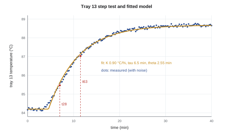
After the 5 % step in steam at \(t = 2\) min, the tray 13 temperature, previously steady at 84.20 °C with about 0.05 °C of noise, does not move for roughly a minute and a half. It then rises in an S-shaped curve and settles near 88.7 °C after about half an hour. The process gain is the steady change divided by the step: \(K = 4.48/5 = 0.90\) °C per percent steam. The shape suggests what the column is physically: the vapor rate rises within seconds of the steam change, but the temperature profile has to shift across several trays before tray 13 feels it, so the response looks like a short dead time followed by a couple of lags.

The first-order-plus-dead-time model

Most self-regulating chemical processes are fitted with the FOPDT model of lesson 3, \(Ke^{-\theta s}/(\tau s + 1)\). It has only three parameters, it captures the two features that matter most for control, the gain and the ratio of dead time to time constant, and nearly every tuning rule in lesson 8 is written in terms of it. A higher-order process fitted with an FOPDT model ends up with a dead time longer than its true transport delay, because the fitted delay absorbs the S-shaped start produced by the smaller lags.

The quickest way to fit it by hand is the two-point method. Find the times after the step at which the response reaches 28.3 % and 63.2 % of its total change, \(t_{28}\) and \(t_{63}\). For a true FOPDT process these are \(\theta + \tau/3\) and \(\theta + \tau\), so

The method is attributed to Smith and is widely used because it needs only two readings from a trend. Its weakness is that both readings come from the noisy part of the curve, and a single bad sample can shift them.

# Fitting a first-order-plus-dead-time model to a step test on the ethanol recovery column
import math, random
random.seed(374)
Kt, t1, t2, tht = 0.90, 6.0, 2.0, 1.0      # the "true" plant (unknown to the engineer): degC per % steam, min
step, t0, dt = 5.0, 2.0, 0.25               # +5 % steam valve at t = 2 min; samples every 15 s
def true(t):
    s = t - t0 - tht
    if s <= 0: return 0.0
    return Kt * step * (1 - (t1 * math.exp(-s / t1) - t2 * math.exp(-s / t2)) / (t1 - t2))
data = [(k * dt, 84.20 + true(k * dt) + random.gauss(0, 0.05)) for k in range(0, 161)]
base = sum(y for t, y in data if t < t0) / len([1 for t, y in data if t < t0])
final = sum(y for t, y in data if t >= 35) / len([1 for t, y in data if t >= 35])
K = (final - base) / step
print(f"baseline {base:.2f} degC, final {final:.2f} degC, gain K = {K:.3f} degC per % steam")
def first_time(frac):
    target = base + frac * (final - base)
    for t, y in data:
        if t > t0 and y >= target: return t - t0
t28, t63 = first_time(0.283), first_time(0.632)
tau_s = 1.5 * (t63 - t28); th_s = t63 - tau_s
print(f"two-point method: t28 = {t28:.2f}, t63 = {t63:.2f} min -> tau = {tau_s:.2f} min, theta = {th_s:.2f} min")
def sse(tau, th):
    s = 0.0
    for t, y in data:
        m = 0.0 if t - t0 < th else K * step * (1 - math.exp(-(t - t0 - th) / tau))
        s += (y - base - m) ** 2
    return s
best = min(((sse(tau, th), tau, th) for tau in [3 + 0.05 * i for i in range(121)] for th in [0.05 * j for j in range(0, 81)]))
print(f"least squares:    tau = {best[1]:.2f} min, theta = {best[2]:.2f} min, rms residual {math.sqrt(best[0] / len(data)):.3f} degC")
print(f"noise added was 0.050 degC; the true plant was second order: tau1 {t1}, tau2 {t2}, dead time {tht} min")
print(f"rule of thumb: the fitted dead time absorbs the smaller lag, theta_fit ~ {tht} + about half of {t2} = {tht + t2 / 2:.1f} min")

baseline 84.20 degC, final 88.68 degC, gain K = 0.896 degC per % steam
two-point method: t28 = 5.00, t63 = 9.50 min -> tau = 6.75 min, theta = 2.75 min
least squares:    tau = 6.50 min, theta = 2.55 min, rms residual 0.076 degC
noise added was 0.050 degC; the true plant was second order: tau1 6.0, tau2 2.0, dead time 1.0 min
rule of thumb: the fitted dead time absorbs the smaller lag, theta_fit ~ 1.0 + about half of 2.0 = 2.0 min

For the tray 13 test, the two-point method gives \(\tau = 6.75\) min and \(\theta = 2.75\) min. A least-squares fit, which adjusts \(\tau\) and \(\theta\) to minimize the squared differences over every sample, gives \(\tau = 6.5\) and \(\theta = 2.55\) min, with a residual of 0.076 °C, close to the 0.05 °C of noise. The two methods agree within about 10 %, which is typical. Theo adopts the least-squares model, rounded: \(K = 0.90\) °C per percent, \(\tau = 6.5\) min, \(\theta = 2.5\) min. Behind the scenes, the simulated plant in the code was second order with lags of 6 and 2 minutes and a true dead time of only 1 minute. The FOPDT fit has absorbed the smaller lag into its dead time, roughly \(1 + 2/2 = 2\) minutes, plus a little more from noise and the shape of the curve. This is normal and harmless for tuning.

Other model forms

Not every process fits an FOPDT model. An integrating process, such as a level with a pumped outflow, is fitted with \(Ke^{-\theta s}/s\): the slope of the ramp divided by the step gives \(K\), and the time before the ramp starts gives \(\theta\). A process that is clearly second order, with a long S-shaped start, can be fitted with two lags plus a dead time, which matters when derivative action is being considered. A process with inverse response, like the reboiler level of lesson 4, needs a zero. The key question is not which model is most accurate, but which is good enough for the controller being designed.

Ratio of dead time to time constant

The single most useful number from a step test is the ratio \(\theta/\tau\), sometimes called the controllability ratio. For tray 13 it is \(2.5/6.5 = 0.38\). Loops with \(\theta/\tau\) below about 0.2 are lag-dominant and easy to control tightly; loops with \(\theta/\tau\) above about 1 are dead-time-dominant, and no feedback controller can respond faster than the dead time allows. Composition loops on slow analyzers often fall into the second group, which is one reason feedforward and model-based control earn their keep there.

Fitting an integrating process

Theo's second test is on the decanter-water surge tank's neighbor, the stripper feed drum, whose outflow is pumped on flow control and whose level therefore integrates. With the outflow held, a 3 % step in the drum's inlet valve makes the level ramp at 0.45 % of span per minute, starting about 0.4 minutes after the step. The integrating model is \(Ke^{-\theta s}/s\) with \(K = 0.45/3 = 0.15\) per minute, the slope per unit step, and \(\theta = 0.4\) min. Such tests must be short, because the level keeps moving; Theo stops this one after six minutes, when the level has risen about 2.5 % of span, and returns the valve. Integrating models are fitted to the slope, not to a final value, and lesson 12 uses them to tune the averaging level controllers.

Pitfalls in plant testing

Theo's test went smoothly, but Malik lists what spoils step tests in practice. A disturbance arriving during the test, such as a feed change or a cooling-water swing, adds a response that is not caused by the step and corrupts the fit; the cure is to repeat the test, or to step in both directions and average. A valve with stiction, sticking until the signal has moved far enough and then jumping, makes the applied step different from the requested one, so the valve position, not the controller output, should be recorded where it is measured. Measurement filters in the transmitter or the DCS add lag that belongs to the loop, and must be included in the model rather than hidden. Nonlinear processes give different gains for steps up and down. Finally, a test done at night at reduced rate may not represent day-time operation.

Modern plants also identify models from routine operating data, using system identification methods that fit models to many small moves, sometimes from pseudo-random signals deliberately added by the control system. Model predictive controllers, lesson 10, are almost always commissioned with models identified this way. The principle is the same: excite the process enough to see its response, and fit the simplest model that reproduces what was seen.

With the model in hand, Theo writes it into the loop's documentation: the date, the operating rate, the size and direction of the step, the fitted gain, time constant and dead time, and the method used. When the loop needs retuning in a year, someone will repeat the test and compare. A drifting gain or a lengthening dead time is often the first sign of fouling, a failing valve, or a change in feed.