
CHE-374 · Lesson 4 of 12 · 20 min
First-order, second-order and dead-time responses
Carla, the panel operator, can glance at a trend and tell Theo what kind of process she is looking at: a smooth approach with no overshoot, a wobble that dies out, a flat line that suddenly starts to move, or a level that first goes the wrong way. Each shape belongs to a family of transfer functions. Recognizing them is the first step in diagnosing a loop and choosing how to control it, and this lesson collects the families that chemical processes produce most often.
First-order processes
A first-order process \(K/(\tau s + 1)\) responds to a step of size \(M\) with \(y(t) = KM(1 - e^{-t/\tau})\). Its signature is a maximum slope at the very start, equal to \(KM/\tau\), followed by a smooth approach. It reaches 63.2 % of its final change at \(t = \tau\), 86.5 % at \(2\tau\), 95 % at \(3\tau\) and 98 % at \(4\tau\). Engineers often say a first-order process has settled after four or five time constants. Single well-mixed tanks, thermal masses and simple flow lags behave this way. If the input is a ramp instead of a step, the output follows the ramp at the same rate but lags behind by exactly \(\tau\) once the transient has died.
Second-order processes
Two first-order lags in series, like the hold tank and transfer line of lesson 3, give an overdamped second-order process: no overshoot, but an S-shaped start. Some second-order processes can oscillate on their own, typically when a mechanical element with inertia is involved, such as a valve actuator or a liquid column in a U-tube manometer. More often in chemical plants, oscillatory second-order behavior appears when a feedback loop is closed. The standard form is
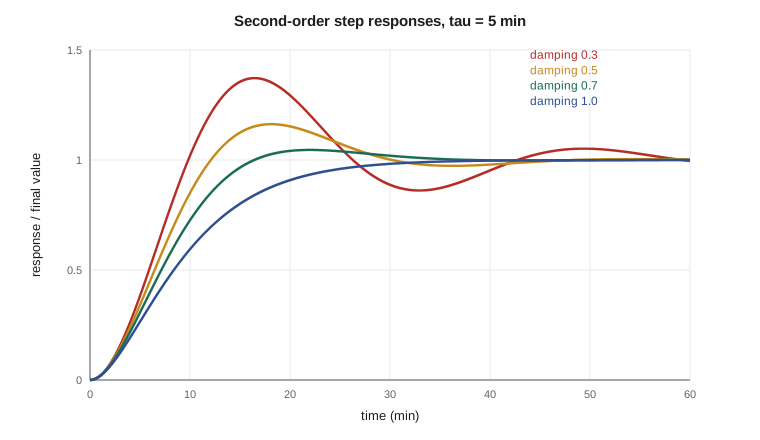
where \(\zeta\) is the damping ratio. For \(\zeta \ge 1\) the response is overdamped; for \(\zeta < 1\) it overshoots and oscillates. The overshoot depends only on \(\zeta\): \(OS = \exp(-\pi\zeta/\sqrt{1 - \zeta^2})\). The decay ratio, the ratio of successive peak heights above the final value, is \(OS^2\), and the period of oscillation is \(2\pi\tau/\sqrt{1 - \zeta^2}\). These formulas let an engineer read a closed-loop trend backwards: measure the overshoot and period, and infer the damping and natural period of the loop.
# Standard responses: second-order behavior, dead time from an analyzer loop, and inverse response
import math
tau = 5.0                                   # min, natural period parameter of a second-order process
print(" zeta  overshoot  decay ratio  period (min)  time to first peak (min)")
for z in (0.3, 0.5, 0.7):
    os_ = math.exp(-math.pi * z / math.sqrt(1 - z * z))
    P = 2 * math.pi * tau / math.sqrt(1 - z * z)
    print(f" {z:.1f}   {100 * os_:6.1f} %   {os_ ** 2:9.3f}   {P:10.1f}   {P / 2:12.1f}")
print(" 1.0 and above: no overshoot (critically damped or overdamped)")
# Dead time of the ester purity analyzer: sample line transport plus a sampling analyzer
L, d, Q = 25.0, 0.004, 0.5                  # m of tubing, m internal diameter, L/min of sample
v = Q / 1000 / 60 / (math.pi * d * d / 4)   # m/s
transport = L / v / 60                      # min
cycle = 4.0                                 # min per chromatographic analysis
theta = transport + cycle + cycle / 2       # result appears one cycle late, sample held on average half a cycle
print(f"sample velocity {v:.2f} m/s, transport {transport:.1f} min; effective dead time about {theta:.1f} min")
# First-order Pade approximation of the dead time, compared on a 10-minute lag
def pade_step(t, th, tl):
    # step response of (1 - th s/2)/(1 + th s/2) / (tl s + 1), by Euler integration
    a, b, x, y = th / 2, tl, 0.0, 0.0; dt = 0.001
    out = []
    for k in range(int(t / dt) + 1):
        # state form of the Pade term: w' = (u - w)/a, z = 2w - u ; then lag: y' = (z - y)/b
        z = 2 * x - 1.0
        out.append(y)
        x += dt * (1.0 - x) / a
        y += dt * (z - y) / b
    return out
tl = 10.0; dt = 0.001; pd = pade_step(30, theta, tl)
print(" t (min)  exact  Pade")
for t in (2, 5, 8, 12, 20, 30):
    exact = 0.0 if t < theta else 1 - math.exp(-(t - theta) / tl)
    print(f" {t:6.0f}  {exact:6.3f}  {pd[int(t / dt)]:6.3f}")
# Inverse response of the reboiler sump level to a steam increase (swell, then fall)
K, a, t1, t2 = -0.20, 4.0, 10.0, 2.0        # m for a 10 % steam step, gravity-drained sump; min
def inv(t):
    # step response of K (1 - a s)/((t1 s + 1)(t2 s + 1))
    c1 = (t1 + a) / (t1 - t2); c2 = (t2 + a) / (t1 - t2)
    return K * (1 - c1 * math.exp(-t / t1) + c2 * math.exp(-t / t2))
ts = [i * 0.05 for i in range(0, 1201)]
ys = [inv(t) for t in ts]
peak = max(ys); tp = ts[ys.index(peak)]
cross = next(t for t, y in zip(ts[1:], ys[1:]) if y < 0)
print(f"sump level first rises {100 * peak:.1f} cm at t = {tp:.1f} min, crosses zero at {cross:.1f} min, settles at {100 * K:.0f} cm") zeta overshoot decay ratio period (min) time to first peak (min)
0.3 37.2 % 0.139 32.9 16.5
0.5 16.3 % 0.027 36.3 18.1
0.7 4.6 % 0.002 44.0 22.0
1.0 and above: no overshoot (critically damped or overdamped)
sample velocity 0.66 m/s, transport 0.6 min; effective dead time about 6.6 min
t (min) exact Pade
2 0.000 -0.088
5 0.000 0.011
8 0.128 0.194
12 0.416 0.427
20 0.737 0.733
30 0.903 0.901
sump level first rises 3.1 cm at t = 1.9 min, crosses zero at 5.0 min, settles at -20 cmWith \(\tau = 5\) min, a damping ratio of 0.3 gives 37 % overshoot and a decay ratio of 0.14; 0.5 gives 16 % and 0.03; 0.7 gives under 5 %. The quarter-decay ratio, \(\zeta \approx 0.21\), was once the standard target for loop tuning, because it gives a fast response. Modern practice, covered in lesson 8, usually prefers damping nearer 0.7, trading a little speed for much more robustness.
| Damping ratio | Overshoot | Decay ratio | Period with tau = 5 min |
|---|---|---|---|
| 0.3 | 37 % | 0.14 | 33 min |
| 0.5 | 16 % | 0.03 | 36 min |
| 0.7 | 4.6 % | 0.002 | 44 min |
| 1.0 | none | - | - |
Dead time
Dead time, or transport delay, is the interval during which the output does not respond at all. In chemical plants it comes from material moving through pipes and equipment before it reaches a sensor, and from analyzers that take time to measure. Transport dead time is volume divided by flow: a 30 m line of 50 mm pipe carrying 6 m³/h holds about 0.06 m³ and delays the signal by roughly 35 seconds. Plug flow through a packed bed or a heat exchanger tube adds similar delays.
Analyzers add more. The ester purity analyzer at Kingfisher Bioenergy is a gas chromatograph fed by a 25 m sample line of 4 mm tubing at 0.5 L/min. The sample travels at 0.66 m/s, so transport takes only about 0.6 min. The chromatograph, however, analyses one sample every 4 minutes and reports the result at the end of its cycle. On average a sample is already half a cycle old when it is taken into the analyzer, and the result appears a full cycle later. The effective dead time is about \(0.6 + 4 + 2 = 6.6\) min, ten times the transport delay. A composition loop on this analyzer cannot react to anything faster than that, which is why the column's main quality loop uses a tray temperature instead, with the analyzer trimming its set point slowly.
Worked problem
Dead time of a transfer line
Ester-rich liquid flows from the decanter to the ester column at 6.0 m³/h through 40 m of 50 mm pipe. Estimate the dead time.
Show solution
- Pipe volume: \(\pi(0.050)^2/4 \times 40 = 0.0785\) m³.
- Flow: \(6.0/60 = 0.10\) m³/min.
- Dead time: \(0.0785/0.10 = 0.79\) min.
Answer: About 47 seconds. At half the flow the dead time doubles, which is one reason loops behave differently at reduced rates.
Approximating dead time
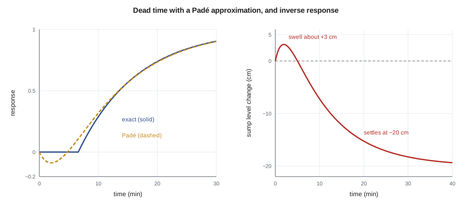
Because \(e^{-\theta s}\) is not a ratio of polynomials, root-locus and some simulation methods replace it with a Padé approximation. The first-order version is \(e^{-\theta s} \approx (1 - \theta s/2)/(1 + \theta s/2)\). It has the right phase at low frequency, but a zero in the right half-plane, so its step response dips the wrong way before rising. The code applies it to a 6.6 min dead time followed by a 10 min lag. At 2 minutes the Padé model shows \(-0.09\) when the exact response is still zero; by 12 minutes the two agree within about 0.01, and later they are indistinguishable. The approximation is good for the overall loop behavior and poor for the detail of the first few minutes.
Inverse response
Some processes first move in the opposite direction to their final change. The classic chemical example is the level in a reboiler or a boiler drum. When the steam to the ester column's reboiler is increased, more liquid boils, and the froth on the tube bundle swells. The level reading rises for a minute or two before the extra vaporization, which removes liquid, makes it fall. Mathematically this is a zero in the right half-plane: \(K(1 - as)/((\tau_1 s + 1)(\tau_2 s + 1))\) with \(a > 0\). With \(K = -0.20\) m for a 10 % steam step, \(a = 4\) min, \(\tau_1 = 10\) and \(\tau_2 = 2\) min, the sump level rises about 3 cm in the first 2 minutes, crosses its starting value at 5 minutes and finally settles 20 cm lower.
Inverse response is a trap for an aggressive controller. A level controller that sees the level rising will cut the steam, which is the right long-term move, but if it reacts hard to the initial swell it will make the swell worse by changing steam again in the wrong phase. Loops with inverse response must be tuned gently, and in drum and reboiler levels the steam is usually not the manipulated variable for level at all; the level is controlled by the bottoms flow, and the steam is left to the temperature loop.
Inverse response also sets a speed limit, much as dead time does. The right-half-plane zero at \(1/a\) adds phase lag at high frequencies without reducing the gain, and a common rule of thumb is that the closed-loop time constant cannot usefully be made shorter than about the inverse-response time \(a\), here 4 minutes, and is often set at two or three times it. Theo writes that limit into the sump level loop's design note, next to the fitted model.
Integrating and unstable processes
The reflux drum of lesson 1 is an integrating process, \(K/s\): a step in its inflow gives a ramp in level that does not stop. Integrators often come with dead time and a small lag, \(Ke^{-\theta s}/(s(\tau s + 1))\). Some processes are open-loop unstable, with a pole in the right half-plane: an exothermic reactor at its middle steady state is one. They cannot be operated without feedback at all, and their control loops must work before the process can be run. Recognizing which family a process belongs to, from a step test or from a model, determines which tuning rules in lesson 8 apply.
Carla's trend-reading habit becomes Theo's checklist. Does the trend move immediately, or after a delay, and how long? Is the start steep or S-shaped? Does it overshoot without control? Does it settle, or keep drifting? Does it begin in the wrong direction? Five questions classify most of what a chemical plant will show him, and each answer narrows the choice of model and of controller.
Common mistakes
MistakeWaiting only one time constant for a first-order process to settle.
InsteadIt has completed 63 %; allow four or five time constants.
MistakeTreating an analyzer's cycle time as negligible.
InsteadA sampling analyzer adds roughly one and a half cycles of dead time.
MistakeTuning a reboiler level loop on steam aggressively.
InsteadInverse response from swell punishes fast action; use the bottoms flow for level.
MistakeTrusting the first moments of a Padé response.
InsteadThe right-half-plane zero makes it dip the wrong way at first.
Summary and key terms
- First-order processes reach 63.2 % at one time constant and about 98 % at four.
- Second-order overshoot depends on damping: 37 % at 0.3, 16 % at 0.5, under 5 % at 0.7.
- Dead time comes from transport and analyzers; the purity analyzer adds about 6.6 min.
- A first-order Padé approximation captures dead time well except in the first minutes.
- Inverse response, from a right-half-plane zero, makes the reboiler level swell before falling.
- Dead time
- The interval after an input change during which the output does not respond.
- Damping ratio
- The parameter that sets how strongly a second-order response oscillates.
- Decay ratio
- The ratio of successive peak heights above the final value in an oscillation.
- Padé approximation
- A ratio of polynomials that approximates a dead time.
- Inverse response
- An initial move opposite to the final change, caused by a right-half-plane zero.
- Swell
- The rise in apparent liquid level when boiling increases in a reboiler or drum.
Practice problems
Work each problem on paper first, then reveal the answer to check.
A first-order process with \(\tau = 8\) min: how long to reach 95 %?
Show answer
About \(3\tau = 24\) min.
An oscillating loop shows 25 % overshoot. Estimate its damping ratio.
Show answer
About 0.4.
A chromatograph cycles every 6 min with negligible transport. Estimate the effective dead time.
Show answer
About \(6 + 3 = 9\) min.
Halve the flow in the decanter-to-column line. What happens to its dead time?
Show answer
It doubles to about 1.6 min.
Write the transfer function of an inverse-response process with a gain of \(-2\), a zero at \(+0.25\) and lags of 10 and 2 min.
Show answer
\(-2(1 - 4s)/((10s + 1)(2s + 1))\).
Why is a column composition loop often built on a tray temperature?
Show answer
The temperature responds in minutes without analyzer delay; the analyzer trims its set point slowly.
Lesson quiz · 5 questions
Score 60% or more to complete this lesson.
Create a free account to save your progress, take quizzes and earn a certificate.