
CHE-374 · Lesson 3 of 12 · 23 min
Laplace transforms and transfer functions
Once Theo has a handful of linear models, Malik wants them in a form that can be connected together like pipes: the heated hold tank feeds a transfer line, the line feeds the reactive column, and a thermowell sits between the liquid and the transmitter. Solving each differential equation in time and then combining the solutions is tedious. The Laplace transform turns linear differential equations into algebra, so that units in series multiply and loops can be closed on paper. Control engineers in every field use it; for chemical processes it is the natural language for lags, dead times and loops.
The transform and its key properties
The Laplace transform of a function of time \(f(t)\), defined for \(t \ge 0\), is \(F(s) = \int_0^\infty f(t) e^{-st}\,dt\), where \(s\) is a complex variable with units of inverse time. Its most useful property for control is what it does to derivatives. If \(f(0) = 0\), the transform of \(df/dt\) is \(sF(s)\). This is why deviation variables matter: by defining every variable as its departure from an initial steady state, all initial values are zero, and a differential equation becomes an algebraic equation in \(s\).
| Time function | Laplace transform | Where it appears |
|---|---|---|
| Unit step, 1 for \(t \ge 0\) | \(1/s\) | A set-point or load change |
| Exponential \(e^{-t/\tau}\) | \(\tau/(\tau s + 1)\) | First-order responses |
| Ramp \(t\) | \(1/s^2\) | A slowly drifting disturbance |
| Derivative \(df/dt\) | \(sF(s) - f(0)\) | Every dynamic balance |
| Integral \(\int_0^t f\,dt\) | \(F(s)/s\) | Levels, integral control |
| Delay \(f(t - \theta)\) | \(e^{-\theta s}F(s)\) | Transport and analyzer dead time |
Applying the transform to the first-order model of lesson 2, \(\tau\,dy/dt + y = Ku\), gives \(\tau s Y(s) + Y(s) = K U(s)\), so
The ratio of output to input transforms, with all initial deviations zero, is the transfer function. It depends only on the process, not on the input. Once it is known, the response to any input is \(Y(s) = G(s)U(s)\), transformed back to time.
Units in series and block diagrams
When the outlet of one unit feeds another and the second does not affect the first, their transfer functions multiply. The heated hold tank, with \(K_p = 0.2045\) K/kW and \(\tau_1 = 22.5\) min, discharges through a jacketed line and a small mixing vessel at the reactive column inlet that together behave like a further lag of 8 minutes. From steam duty to the column inlet temperature:
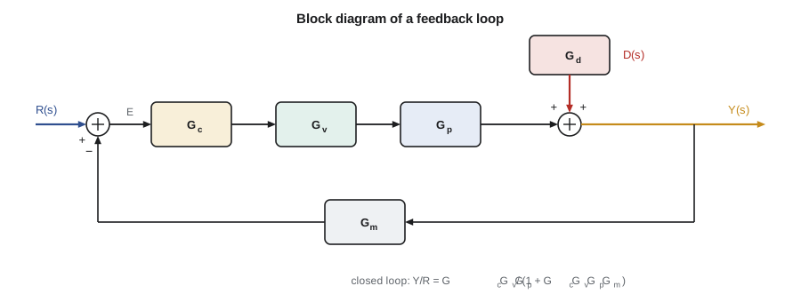
Block diagrams draw each transfer function as a box, with arrows for signals and circles for summing points. Three rules cover most manipulations: blocks in series multiply; blocks in parallel add; and a negative feedback loop with forward path \(G\) and feedback path \(H\) reduces to \(G/(1 + GH)\). Lesson 6 uses the last rule to find the closed-loop response of a controlled process.
Back to time: partial fractions
For a 20 kW step, \(U(s) = 20/s\), and \(Y(s) = 0.2045 \times 20/(s(22.5 s + 1)(8 s + 1))\). Splitting this into partial fractions, each a term from the table, and transforming back gives
The code compares this formula with a direct numerical simulation of the two lags; they agree to three decimal places. Note the shape: unlike a single lag, the response starts with zero slope, because the second lag has not yet received any change from the first. Two or more lags in series produce the S-shaped response typical of real processes, and that shape is why step tests in lesson 5 are fitted with a dead time as well as a time constant.
# Transfer functions: two first-order lags in series, checked by partial fractions and by simulation
import math, cmath
Kp, t1, t2 = 0.2045, 22.5, 8.0       # K/kW (lesson 2), minutes
Q = 20.0                             # kW steam step
K = Kp * Q                           # temperature change for the step, K
def analytic(t):                     # inverse Laplace transform of K / (s (t1 s + 1)(t2 s + 1))
    return K * (1 - (t1 * math.exp(-t / t1) - t2 * math.exp(-t / t2)) / (t1 - t2))
x1 = x2 = 0.0; dt = 0.01; sim = []
for k in range(int(120 / dt) + 1):
    if k % int(20 / dt) == 0: sim.append((k * dt, x2))
    x1 += dt * (K - x1) / t1
    x2 += dt * (x1 - x2) / t2
print("  t (min)  partial fractions  simulation")
for t, y in sim: print(f"  {t:6.0f}  {analytic(t):12.3f}  {y:14.3f}")
print(f"final value theorem: lim s->0 of s * G(s) * Q/s = Kp * Q = {K:.2f} K")
def roots(c, n=200):
    # Durand-Kerner: all roots of c[0] s^n + c[1] s^(n-1) + ... + c[n]
    c = [x / c[0] for x in c]; deg = len(c) - 1
    r = [complex(0.4, 0.9) ** k for k in range(deg)]
    for _ in range(n):
        new = []
        for i, ri in enumerate(r):
            num = sum(ck * ri ** (deg - k) for k, ck in enumerate(c))
            den = 1
            for j, rj in enumerate(r):
                if j != i: den *= ri - rj
            new.append(ri - num / den)
        r = new
    return r
den = [t1 * t2, t1 + t2, 1.0]          # (t1 s + 1)(t2 s + 1)
print("poles of G:", ", ".join(f"{p.real:.4f}" for p in sorted(roots(den), key=lambda z: z.real)), "1/min")
# Add a third lag of 3 min (a thermowell) and close a proportional loop: 1 + Kc G = 0
t3 = 3.0
for Kc in (10.0, 40.0, 80.0):
    a = [t1 * t2 * t3, t1 * t2 + t1 * t3 + t2 * t3, t1 + t2 + t3, 1 + Kc * Kp]
    ps = roots(a)
    worst = max(p.real for p in ps)
print(f"Kc = {Kc:4.0f} kW/K: closed-loop poles " + ", ".join(f"{p.real:+.3f}{p.imag:+.3f}j" for p in ps) + (" stable" if worst < 0 else " UNSTABLE".lower())) t (min) partial fractions simulation
0 0.000 0.000
20 1.666 1.667
40 3.033 3.033
60 3.650 3.651
80 3.909 3.909
100 4.015 4.016
120 4.059 4.059
final value theorem: lim s->0 of s * G(s) * Q/s = Kp * Q = 4.09 K
poles of G: -0.1250, -0.0444 1/min
Kc = 10 kW/K: closed-loop poles -0.062-0.105j, -0.062+0.105j, -0.378+0.000j stable
Kc = 40 kW/K: closed-loop poles -0.027-0.193j, -0.027+0.193j, -0.449+0.000j stable
Kc = 80 kW/K: closed-loop poles +0.002-0.252j, +0.002+0.252j, -0.506+0.000j unstableThe final value theorem
Often only the end point is wanted. The final value theorem states that if \(y(t)\) settles, its final value is \(\lim_{s \to 0} sY(s)\). For a step of size \(M\) into \(G(s)\), the final value is \(M\,G(0)\), the steady-state gain times the step. For the hold tank and line, \(G(0) = 0.2045\) K/kW, so a 20 kW step gives 4.09 K, as the simulation shows. The theorem only applies if the response actually settles; applied to an unstable system it returns a meaningless number, so stability must be checked first.
Worked problem
Final value of a controlled process
A proportional controller \(K_c\) acts on \(G(s) = K/(\tau s + 1)\) in a loop with unit feedback. Find the steady offset after a unit set-point step.
Show solution
- Closed loop: \(Y/R = K_cG/(1 + K_cG) = K_cK/(\tau s + 1 + K_cK)\).
- Final value: \(\lim_{s\to 0} s \cdot (1/s) \cdot K_cK/(\tau s + 1 + K_cK) = K_cK/(1 + K_cK)\).
- Offset \(= 1 - K_cK/(1 + K_cK) = 1/(1 + K_cK)\).
Answer: The offset is \(1/(1 + K_cK)\), the formula lesson 6 checks by simulation.
Poles, zeros and stability
A transfer function is usually a ratio of polynomials in \(s\). The roots of the denominator are the poles; the roots of the numerator are the zeros. Each pole contributes a term \(e^{pt}\) to the response. A negative real pole gives a decaying exponential; a pair of complex poles with negative real parts gives a decaying oscillation; any pole with a positive real part gives a response that grows without bound. A linear system is stable if and only if all its poles lie in the left half of the complex plane. The hold tank and line have poles at \(-1/22.5 = -0.044\) and \(-1/8 = -0.125\) min\(^{-1}\): both negative, both real, so the open-loop response is a smooth approach to the final value.
Closing a loop moves the poles. With a proportional controller on the hold tank, line and a 3-minute thermowell, the closed-loop poles are the roots of \(1 + K_cG(s) = 0\), a cubic. The code finds them with the Durand-Kerner method. At \(K_c = 10\) kW/K the dominant pair is complex with real part \(-0.062\): an oscillatory but well-damped response. At 40 kW/K the real part has shrunk to \(-0.027\), so oscillations die slowly. At 80 kW/K the pair has crossed into the right half-plane and the loop is unstable: any disturbance grows into a sustained, growing oscillation until the steam valve hits its limits. Lesson 7 finds the boundary exactly, at 77.5 kW/K.
A worked transfer function for the surge tank
Lesson 2's linearized surge tank, \(\tau\,dh'/dt + h' = Kq'\) with \(\tau = 45\) min and \(K = 0.25\) m per m³/h, transforms to \(H(s)/Q(s) = 0.25/(45s + 1)\). Suppose the stripper downstream is fed from this tank and its feed controller is slow, so the tank outflow can be treated as set by the level alone. A ramp in inflow, as when the decanter is slowly raising its rate at 0.1 m³/h per minute, has the transform \(0.1/s^2\). The level is then \(H(s) = 0.025/(s^2(45s + 1))\). Partial fractions give \(h'(t) = 0.025\big(t - 45 + 45e^{-t/45}\big)\) m, with \(t\) in minutes: after the initial transient, the level rises at 0.025 m per minute, lagging the steady-state relationship by one time constant. Theo uses exactly this result to check how long the tank can absorb a ramped rate change before its high-level alarm, 0.6 m above normal, is reached: just under an hour.
Worked problem
Time to reach an alarm on a ramp
Using \(h'(t) = 0.025(t - 45 + 45e^{-t/45})\) m, estimate when the level reaches 0.6 m above normal.
Show solution
- For \(t\) well above 45 min the exponential is small, so \(h' \approx 0.025(t - 45)\).
- Setting \(0.025(t - 45) = 0.6\) gives \(t = 69\) min.
- Check: at 69 min, \(e^{-69/45} = 0.22\), adding \(0.025 \times 45 \times 0.22 = 0.25\) m, so the true level is higher and the alarm comes sooner; solving exactly gives about 56 min.
Answer: About an hour. The transfer function turns a question about an operating procedure into two lines of algebra.
Dead time in the s-domain
A pure delay of \(\theta\) has the transfer function \(e^{-\theta s}\). It is not a ratio of polynomials, which complicates root-finding, but it fits naturally into frequency-response methods, where \(s = j\omega\) and \(e^{-j\omega\theta}\) simply adds a phase lag of \(\omega\theta\) radians. The standard model for chemical processes, the first-order-plus-dead-time or FOPDT model, is \(K e^{-\theta s}/(\tau s + 1)\). Lessons 4 to 8 rely on it heavily. Where a polynomial form is needed, the delay is replaced by a Padé approximation, shown in lesson 4.
Theo notes one practical warning from Malik: the algebra of transfer functions assumes linear, time-invariant behavior. Valves that saturate, controllers that switch modes, and processes whose gain changes with rate all break that assumption. Transfer functions are the right tool for understanding and tuning a loop near its operating point; they are not a substitute for simulating a large upset.
Transfer functions also tidy up how a plant is described in documents. Instead of a page of differential equations, the design file for a loop can carry one line: tray temperature to steam flow, \(0.9e^{-2.5s}/(6.5s + 1)\) °C per percent, minutes, measured on a given date at a given rate. Anyone can read off the gain, the lag and the dead time, compare them with a later test, and see at once whether the process has changed. Theo starts keeping such a line for every loop he works on.
Common mistakes
MistakeTaking the transform with non-zero initial values and dropping them.
InsteadUse deviation variables so that every initial value is zero.
MistakeMultiplying transfer functions of units that interact.
InsteadSeries multiplication assumes the downstream unit does not affect the upstream one.
MistakeApplying the final value theorem to an unstable loop.
InsteadCheck that all poles are in the left half-plane first.
MistakeReading a single lag's step response shape into a multi-lag process.
InsteadLags in series give an S-shaped start with zero initial slope.
Summary and key terms
- The Laplace transform turns linear differential equations in deviation variables into algebra.
- A transfer function is the ratio of output to input transforms; series blocks multiply.
- Partial fractions return a transform to time; the final value theorem gives \(M\,G(0)\) for a step.
- Poles decide stability: all must have negative real parts.
- Raising proportional gain moved the hold-tank loop's poles into the right half-plane above about 78 kW/K.
- Laplace transform
- An integral transform that maps functions of time to functions of a complex variable s.
- Transfer function
- The ratio of the transforms of output and input, with zero initial deviations.
- Pole
- A root of the denominator of a transfer function; it sets a mode of the response.
- Zero
- A root of the numerator of a transfer function.
- Final value theorem
- The rule that a settling response tends to the limit of sY(s) as s tends to zero.
- Block diagram
- A drawing of signals and transfer functions connected by arrows and summing points.
Practice problems
Work each problem on paper first, then reveal the answer to check.
Find the transfer function of \(5\,dy/dt + y = 2u\).
Show answer
\(G = 2/(5s + 1)\).
What is the final value of a 3-unit step into \(4/((2s + 1)(s + 1))\)?
Show answer
\(3 \times 4 = 12\).
Give the poles of \(1/(s^2 + 3s + 2)\).
Show answer
\(-1\) and \(-2\).
Reduce a loop with forward path \(G = 2/(s + 1)\) and unit feedback.
Show answer
\(G/(1 + G) = 2/(s + 3)\).
Why does a two-lag process start with zero slope?
Show answer
The second lag receives no change until the first has started to respond.
A pole lies at \(+0.01\) min\(^{-1}\). After how long does its mode grow by a factor of \(e\)?
Show answer
100 min.
Lesson quiz · 5 questions
Score 60% or more to complete this lesson.
Create a free account to save your progress, take quizzes and earn a certificate.