Multivariable control and model predictive control

The ester column of CHE-350 has two quality targets: its bottoms must be 99.9 wt % ester, and its distillate must stay close to the ternary azeotrope so that the recycle to the decanter does not carry extra ester. Each end has a sensitive tray, tray 5 near the top and tray 22 near the bottom, and the obvious design is two loops: reflux controls tray 5, boil-up controls tray 22. When Theo puts both loops in automatic on the training simulator, they fight. A correction at the top upsets the bottom, the bottom loop responds, which upsets the top, and the column rings for an hour. He has met interaction, the defining problem of multivariable control.

Interaction and the relative gain array

In a column, almost every manipulated variable affects almost every controlled variable. More reflux cools the whole column, not only the top; more boil-up heats the whole column, not only the bottom. A step test with each manipulated variable in turn gives a matrix of steady-state gains. For the ester column, in °C per percent, with reflux \(L\) and boil-up \(V\) (illustrative values from the rigorous model):

Bristol's relative gain array, RGA, measures how much the other loops change each pairing. Its element \(\lambda_{ij}\) is the gain from input \(j\) to output \(i\) with all other loops open, divided by the same gain with all other loops closed and holding their outputs constant. For a 2 by 2 system, \(\lambda_{11} = 1/(1 - g_{12}g_{21}/(g_{11}g_{22}))\), and each row and column of the array sums to 1. A relative gain of 1 means the other loop has no effect on this pairing. A value between 0.5 and 1 means mild interaction. Values well above 1 mean the other loop opposes this one, so it must work harder once both are closed. Negative values mean the pairing reverses its sign when the other loop is closed, and must be avoided.

# Interaction in the ester column (relative gain array) and a small dynamic matrix controller
import math
def rga2(g):
    l = 1 / (1 - g[0][1] * g[1][0] / (g[0][0] * g[1][1]))
    return l
LV = ((-0.80, 0.95), (-0.55, 1.20))       # tray temperatures T5 (top), T22 (bottom) vs reflux L, boil-up V; degC per %
DV = ((0.80, 0.25), (0.55, 0.95))         # same outputs vs distillate D and boil-up V (illustrative)
for name, g in (("LV", LV), ("DV", DV)):
    l = rga2(g); det = g[0][0] * g[1][1] - g[0][1] * g[1][0]
    print(f"{name} configuration: lambda11 = {l:.2f}, RGA rows ({l:.2f}, {1 - l:.2f}) and ({1 - l:.2f}, {l:.2f}), Niederlinski index {det / (g[0][0] * g[1][1]):.2f}")
# Static decoupler for LV: with D21 = -g21/g22, a reflux move is followed by a boil-up move that cancels its effect on T22
d21 = -LV[1][0] / LV[1][1]
print(f"decoupler: for each 1 % reflux move, add {d21:+.3f} % boil-up; T5 gain then becomes {LV[0][0] + LV[0][1] * d21:+.3f} degC per %")
# Dynamic matrix control of the tray temperature (FOPDT K 0.90, tau 6.5, theta 2.5), sample time 0.5 min
K, tau, th, Ts = 0.90, 6.5, 2.5, 0.5
N, P, M = 80, 20, 3
a = [0.0 if (i + 1) * Ts <= th else K * (1 - math.exp(-((i + 1) * Ts - th) / tau)) for i in range(N)]
def solve(A, b):
    n = len(b); A = [row[:] + [b[i]] for i, row in enumerate(A)]
    for c in range(n):
        p = max(range(c, n), key=lambda r: abs(A[r][c])); A[c], A[p] = A[p], A[c]
        for r in range(n):
            if r != c:
                f = A[r][c] / A[c][c]; A[r] = [x - f * y for x, y in zip(A[r], A[c])]
    return [A[i][n] / A[i][i] for i in range(n)]
def dmc(lam, maxmove=None, steps=80):
    Dyn = [ [a[i - j] if i >= j else 0.0 for j in range(M)] for i in range(P)]
    H = [ [sum(Dyn[k][i] * Dyn[k][j] for k in range(P)) + (lam if i == j else 0.0) for j in range(M)] for i in range(M)]
    du_hist = [0.0] * N; u = 0.0; ys = []
    true_y = 0.0
    for k in range(steps):
        # free response: effect of past moves only (the model is taken as perfect here)
        free = []
        for i in range(1, P + 1):
            s = 0.0
            for j, du in enumerate(du_hist):
                idx = min(N - 1, i + j)
                s += a[idx] * du
            free.append(s)
        err = [1.0 - f for f in free]
        g = [sum(Dyn[r][i] * err[r] for r in range(P)) for i in range(M)]
        move = solve(H, g)[0]
        if maxmove is not None: move = max(-maxmove, min(maxmove, move))
        du_hist = [move] + du_hist[:-1]; u += move
        true_y = sum(a[min(N - 1, j)] * du for j, du in enumerate(du_hist))
        ys.append((k * Ts, true_y, u))
    return ys
for lam in (0.1, 1.0, 5.0):
    ys = dmc(lam)
    peak = max(y for t, y, u in ys); umax = max(u for t, y, u in ys)
    t95 = next(t for t, y, u in ys if y >= 0.95)
    print(f"DMC, move suppression {lam:3.1f}: first reaches 95 % at {t95:4.1f} min, overshoot {100 * max(0, peak - 1):4.1f} %, peak steam move {umax:5.2f} %")
ys = dmc(0.1, maxmove=0.4)
print(f"with moves limited to 0.4 % per 30 s: reaches 95 % at {next(t for t, y, u in ys if y >= 0.95):.1f} min")

LV configuration: lambda11 = 2.19, RGA rows (2.19, -1.19) and (-1.19, 2.19), Niederlinski index 0.46
DV configuration: lambda11 = 1.22, RGA rows (1.22, -0.22) and (-0.22, 1.22), Niederlinski index 0.82
decoupler: for each 1 % reflux move, add +0.458 % boil-up; T5 gain then becomes -0.365 degC per %
DMC, move suppression 0.1: first reaches 95 % at  5.5 min, overshoot  2.5 %, peak steam move  3.38 %
DMC, move suppression 1.0: first reaches 95 % at  9.5 min, overshoot  0.1 %, peak steam move  1.95 %
DMC, move suppression 5.0: first reaches 95 % at 11.0 min, overshoot  0.9 %, peak steam move  1.65 %
with moves limited to 0.4 % per 30 s: reaches 95 % at 7.5 min

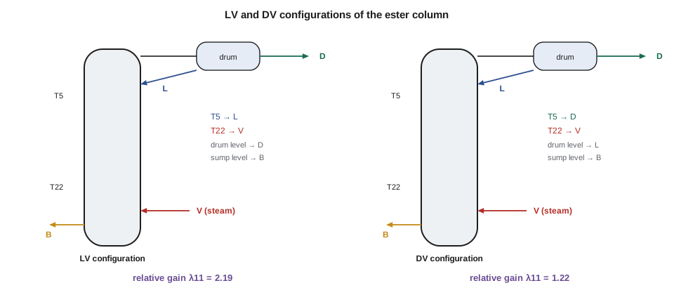
For the LV configuration, \(\lambda_{11} = 2.19\). Pairing reflux with tray 5 and boil-up with tray 22 is the right way round, since the diagonal elements are positive, but the interaction is strong: closing the tray 22 loop reduces the effective gain of reflux on tray 5 to less than half its open-loop value, and vice versa. The Niederlinski index, \(\det(G)/(g_{11}g_{22}) = 0.46\), is positive, so the pairing will not be unstable for structural reasons, but it will be sluggish and oscillatory unless the loops are tuned with that in mind.

Changing the configuration

Column engineers have long known that the choice of manipulated variables matters as much as the tuning. Instead of reflux, the top composition can be controlled with the distillate flow \(D\), letting the reflux drum level controller set the reflux. In this DV configuration the illustrative gain matrix gives \(\lambda_{11} = 1.22\) and a Niederlinski index of 0.82: much weaker interaction. The physical reason is that a change in distillate changes the column's material balance, which affects mainly one end, while reflux and boil-up both change the internal flows and move both ends together. Other configurations, such as ratios of reflux to distillate or boil-up to bottoms, sometimes do better still. Choosing among them is part of the capstone in lesson 12.

Decoupling

If interaction cannot be avoided by choosing a better configuration, a decoupler can cancel it. A static decoupler for the LV column adds, to each reflux move, a boil-up move that leaves tray 22 unchanged: \(D_{21} = -g_{21}/g_{22} = +0.46\) % boil-up per % reflux. The tray 5 controller then sees an effective gain of \(-0.80 + 0.95 \times 0.46 = -0.37\) °C per percent, since the compensating boil-up move works against the reflux at the top. Decouplers work well when the gain matrix is well known and fairly constant. They become fragile when the RGA elements are large, because small model errors are then amplified, which is also when they would be most useful. That observation was one of the motivations for the next approach.

Model predictive control

Model predictive control, MPC, takes a different approach to multivariable problems. Instead of pairing inputs with outputs, it uses a dynamic model of the whole unit to predict how every controlled variable will move over a horizon into the future, and chooses a sequence of moves in every manipulated variable that brings the predictions to their targets while respecting limits on valves, rates of change and process constraints. At each control interval, typically a minute in chemical plants, it applies only the first move, measures the plant again, corrects its prediction, and repeats. This receding-horizon idea gives MPC its feedback.

The first industrial MPC, dynamic matrix control, or DMC, was developed at Shell in the late 1970s. It uses step-response models, the very curves measured in lesson 5, stored as lists of coefficients. Predicting the effect of future moves is then a matrix multiplication, and choosing the moves is a least-squares problem: minimize the squared prediction errors plus a penalty, the move suppression, on the size of the moves. Modern products add constraints, solved by quadratic programming, and steady-state economic optimization of the targets.

The code builds a small DMC for tray 13 alone, using the FOPDT model sampled every 30 seconds, an 80-coefficient step response, a 20-step prediction horizon and 3 future moves. With light move suppression, \(\lambda = 0.1\), the temperature reaches 95 % of a 1 °C set-point change in 5.5 minutes, with 2.5 % overshoot, and the steam moves 3.4 % at its peak. Heavier suppression, \(\lambda = 1\), takes 9.5 minutes, with almost no overshoot and only 2 % steam movement. Move suppression is MPC's main tuning knob: it trades speed for smooth valve action and robustness to model error. Limiting each move to 0.4 % per interval, a typical rate constraint, the controller still reaches 95 % in 7.5 minutes by spreading its moves out.

MPC in practice at the plant

At Kingfisher Bioenergy, MPC runs on top of the regulatory loops, not in place of them. The ethanol distillation and dehydration section has one controller with six manipulated variables, all of them set points of existing PID loops such as steam flows, reflux flows and feed rate, and about fifteen controlled and constraint variables: tray temperatures, analyzer readings, column pressure drops, valve positions and the molecular sieve cycle. Its models were identified from a two-week step-testing campaign. It pushes the units toward their most profitable constraint, usually the steam supply or the dehydration capacity, and the benefit, a few percent more throughput and lower steam per liter, paid for it within a year.

Above MPC, real-time optimization uses a steady-state model of the plant, often a full process simulator, to choose economic targets every few hours: how hard to push the beer column given today's steam cost, or what purity to aim for when the ester price changes. Theo notices that each layer is slower and more model-based than the one below, and that each one depends on the layers beneath it working well. An MPC moving the set point of an oscillating PID loop inherits the oscillation.

Malik is candid about MPC's costs. It needs good models, re-identified when the plant changes. It needs engineers who understand it, because operators turn off controllers they cannot predict. And it does not remove the need for sound regulatory control. Most of the benefit of an MPC project, he says, often comes from fixing the PID loops and valves during the preparation.