Data-level parallelism: SIMD, vectors, GPUs and accelerators

Many important workloads apply the same operation to large amounts of data: filtering a radar signal, transforming an image, multiplying matrices in a neural network. This data-level parallelism is far cheaper to exploit than the instruction-level parallelism of lessons 5 and 6, because one instruction can command many operations at once, so the costs of fetching, decoding and scheduling are shared among them. Vector processors, packed SIMD instructions, graphics processing units and domain-specific accelerators all exploit it in different ways. As general-purpose cores have hit power limits, these specialized forms of parallelism have become the main source of new performance in everything from phones to data centres.

The NS-5 classifier is mostly data-parallel arithmetic: a filter over each radar frame, a fast Fourier transform to measure range, and a small convolutional neural network that labels the vehicle. Core B offers packed SIMD instructions; a third option, Core B plus a small integer neural network accelerator, has appeared in a vendor's catalogue. Maren asks Jonah how much each would help, and the honest answer requires a model of when computation, not memory, is the bottleneck.

Flynn's taxonomy and SIMD

A classic classification divides computers by their instruction and data streams. SISD, single instruction single data, is the ordinary scalar processor. SIMD, single instruction multiple data, applies one instruction to many data elements. MIMD, multiple instruction multiple data, is the multicore processor of lesson 10, with independent instruction streams. MISD has no common practical form. Every form of data-level parallelism in this lesson is a kind of SIMD, differing in how wide the data are, how the hardware is organized, and how software expresses the parallelism.

Packed SIMD extensions

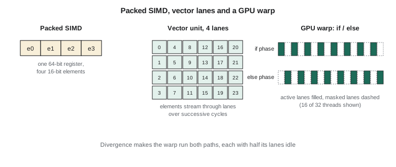
The simplest form treats a wide register as several narrow elements. A 64-bit register can hold four 16-bit samples, and a packed add adds all four pairs at once. Packed SIMD extensions were added to desktop instruction sets from the 1990s onward, growing from 64-bit to 128-, 256- and 512-bit registers. They are cheap to add to an existing datapath, but they have drawbacks: each new register width brings a new set of instructions, code written for one width does not use a wider one, loops whose lengths are not multiples of the width need extra cleanup code, and loading data that are not aligned or not contiguous is awkward. Core B's packed instructions process two 16-bit or four 8-bit values in its 32-bit registers, which roughly quadruples peak throughput on byte-sized data.

Vector architectures and the RISC-V V extension

True vector architectures, which date back to the supercomputers of the 1970s, avoid these problems by making the vector length a run-time quantity. The RISC-V V extension provides 32 vector registers, each VLEN bits long, where VLEN is chosen by the implementation, from 128 bits in small cores to thousands of bits in large ones. Software asks for a vector length with the vsetvli instruction, stating the element width and the number of elements remaining, and the hardware replies with how many it will process this time, up to its capacity. A loop processes that many elements, advances its pointers, and repeats, a technique called strip-mining. The same binary therefore runs on any implementation and automatically uses its full width, and the final partial strip needs no special code.

Vector instructions also include strided loads, which gather every kth element, indexed gathers and scatters, which follow a vector of addresses, and masks, which let each element of an operation be enabled or disabled so that conditional code can be vectorized. Vector units are deeply pipelined: a long vector operation streams its elements through the functional units over several cycles, and chaining lets a dependent vector operation start on the first elements before the previous one has finished. Multiple lanes, each a slice of the datapath handling a subset of elements, give the hardware parallelism.

# y[i] = y[i] + c * x[i] for n int16 samples using RISC-V vectors
# a0 = n, a1 = &x, a2 = &y, a3 = c
loop:
    vsetvli  t0, a0, e16, m1, ta, ma   # t0 = elements this pass (up to VLEN/16)
    vle16.v  v1, (a1)                  # load t0 elements of x
    vle16.v  v2, (a2)                  # load t0 elements of y
    vmacc.vx v2, a3, v1                # v2 += c * v1, element by element
    vse16.v  v2, (a2)                  # store y
    slli     t1, t0, 1                 # bytes processed = 2 * t0
    add      a1, a1, t1
    add      a2, a2, t1
    sub      a0, a0, t0                # elements remaining
    bnez     a0, loop

Graphics processing units

GPUs grew from fixed graphics pipelines into general-purpose data-parallel processors. Their programming model presents the work as thousands of lightweight threads, each running the same kernel program on its own data element. The hardware groups threads into warps of typically 32, which execute in lockstep on SIMD lanes: one instruction is fetched and issued for the whole warp, and each lane applies it to its own thread's registers. This style is often called SIMT, single instruction multiple threads. A GPU contains dozens of multiprocessors, each holding many warps at once; when one warp stalls on a memory access, the scheduler switches to another ready warp in the next cycle. GPUs hide memory latency with massive multithreading rather than with large caches and out-of-order execution, which lets them devote most of their area to arithmetic.

Lockstep execution has a cost when threads in a warp disagree at a branch. The warp must execute both paths, masking off the lanes that did not take each one, so if half the threads take the if path and half the else path, the warp spends the time of both paths with each lane idle half the time. This branch divergence, together with uncoalesced memory accesses, in which the threads of a warp touch scattered addresses instead of consecutive ones, is the main reason GPU programs fall short of their peak.

The roofline model

Whether a data-parallel machine can reach its peak depends on how much computation each byte of data supports. The arithmetic intensity of a kernel is the number of operations it performs per byte moved to or from memory. The roofline model plots attainable performance against arithmetic intensity: below a certain intensity, performance is limited by memory bandwidth, rising in proportion to intensity; above it, performance is capped by the peak compute rate. The bend in the roof, the ridge point, is the intensity at which a machine becomes compute-bound.

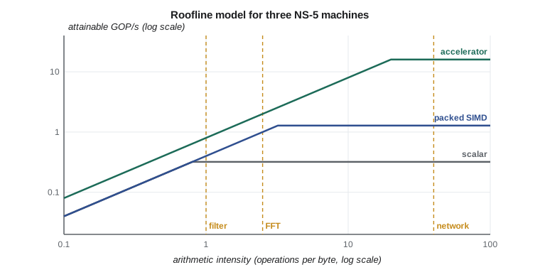
The model tells an architect which improvements can help. A kernel to the left of the ridge gains nothing from more arithmetic units; it needs more bandwidth, better caching to raise its effective intensity, or data in narrower formats. A kernel to the right gains from wider SIMD or an accelerator. Jonah estimates the intensity of the three NS-5 kernels from their code and compares three machines: Core B using scalar instructions, Core B using its packed instructions, and Core B with the integer accelerator, which comes with a slightly faster memory interface. The peak and bandwidth figures are from vendor datasheets and are approximate.

# Roofline estimates for NS-5 kernels, vector strip-mining and GPU branch divergence
def attainable(peak_gops, bw_gbs, intensity):
    return min(peak_gops, bw_gbs * intensity)

machines = {"Core B scalar": (0.32, 0.4), "Core B packed SIMD": (1.28, 0.4), "int8 accelerator": (16.0, 0.8)}
kernels = {"FIR filter (int16)": 1.0, "range FFT": 2.5, "CNN layer (int8)": 40.0}   # operations per byte
print("kernel                 intensity " + "".join(f"{m:>20s}" for m in machines))
for k, ai in kernels.items():
    row = "".join(f"{attainable(p, b, ai):17.2f} G" + ("*" if b * ai < p else " ") + " " for p, b in machines.values())
    print(f"{k:22s} {ai:6.1f}   {row}")
print("* = memory-bound at this intensity")

# Strip-mining a 2048-element loop on a vector unit with VLEN = 128 bits and 16-bit elements
vlen_bits, sew, n = 128, 16, 2048
vl_max = vlen_bits // sew
passes = -(-n // vl_max)
print(f"elements per vector instruction: {vl_max}, loop passes: {passes} (scalar loop: {n})")

# GPU warps of 32 threads: an if/else where threads take different paths
def efficiency(fraction_taken, warp=32):
    taken = round(fraction_taken * warp)
    paths = (taken > 0) + (taken < warp)       # number of paths the warp must execute
    return 1 / paths
for f in (0.0, 1 / 32, 0.5, 1.0):
    print(f"fraction taking the if-branch {f:5.3f}: SIMD efficiency {efficiency(f):.2f}")

kernel                 intensity        Core B scalar  Core B packed SIMD    int8 accelerator
FIR filter (int16)        1.0                0.32 G               0.40 G*              0.80 G* 
range FFT                 2.5                0.32 G               1.00 G*              2.00 G* 
CNN layer (int8)         40.0                0.32 G               1.28 G              16.00 G  
* = memory-bound at this intensity
elements per vector instruction: 8, loop passes: 256 (scalar loop: 2048)
fraction taking the if-branch 0.000: SIMD efficiency 1.00
fraction taking the if-branch 0.031: SIMD efficiency 0.50
fraction taking the if-branch 0.500: SIMD efficiency 0.50
fraction taking the if-branch 1.000: SIMD efficiency 1.00

The table shows why accelerators are not a universal answer. The filter performs about one operation per byte, so it is memory-bound on every machine except the scalar core: packed SIMD improves it only from 0.32 to 0.40 billion operations per second, and the accelerator helps only because of its faster memory interface. The FFT, at 2.5 operations per byte, is also memory-bound once packed or accelerated. The neural network layer, which reuses each weight and activation many times, has high intensity and gains the full benefit: 1.28 billion operations per second with packed SIMD and 16 with the accelerator, a factor of 50 over scalar code. The strip-mining line shows that a 128-bit vector unit would process the 2,048-sample frame in 256 passes instead of 2,048 iterations, and the divergence lines show that a single thread taking a different path halves a warp's efficiency just as much as an even split does.

Domain-specific accelerators

When a workload is important enough, designers build hardware for it alone. Domain-specific architectures follow a few principles: use dedicated memories, such as scratchpads managed by software, instead of general caches, to minimize data movement; spend area on many simple arithmetic units instead of on prediction and speculation; use the narrowest data types the application tolerates, such as 8-bit integers or even narrower formats for neural network inference; and program them through a domain-specific language or library that exposes their parallelism. Neural network accelerators, often built as systolic arrays in which data flow rhythmically through a grid of multiply-accumulate units, can reach tens to hundreds of times the performance per watt of a general-purpose core on their target workload.

Specialization trades flexibility for efficiency. An accelerator designed for one generation of neural networks may suit the next poorly, software support takes effort, and silicon area spent on a unit that is idle most of the time is wasted. For the NS-5, the integer accelerator would make the network layer, about 70 percent of Core B's classifier time, at least eight times faster on its own, and lesson 1's Amdahl calculation suggests an overall gain of about 2.6 times. Whether that justifies its area, its 9 mW of extra active power and its software toolchain is a question for the trade study in lesson 12.