
CMP-310 · Lesson 1 of 12 · 21 min
Quantitative design and computer performance
Computer organization explained how a processor executes a program: how instructions are encoded, how a datapath moves values between registers and memory, and how a simple pipeline and cache work. Computer architecture asks the designer's question instead. Given a power budget, a cost target, a workload and a technology, which processor and memory system should we build, and how do we know it is better than the alternatives? Answering that question needs numbers. Architects measure, model and compare before they commit to silicon or to a purchase order, because a choice that looks clever on a whiteboard can waste energy, money and months of firmware effort.
This course continues at Northway Sensing in Kingston, Ontario, maker of the NS-4 solar-powered roadside traffic counter. Jonah Abara, now a third-year co-op student, has joined a small team planning the next node, the NS-5. Maren Holt, the firmware lead, owns the decision about which processor core and memory system the NS-5 will use, and Dana Okoye from the server team brings questions about the machines that store and process the counts. The NS-5 must classify vehicles from a radar sensor on the node itself instead of sending raw data to the server, so for the first time the processor's performance and energy really matter.
CMP-229 Computer Organization covered the single-cycle datapath, the basic five-stage pipeline, direct-mapped caches and the idea of virtual memory. This course assumes that background and goes further: how pipelines are made to approach one instruction per cycle and beyond, how processors execute instructions out of order and in parallel, how cache hierarchies are tuned, how virtual memory protects programs, how many cores share memory correctly, and how vector units, GPUs and accelerators gain their speed. It ends with a design trade study for the NS-5.
What 'faster' means
Two numbers dominate performance discussions. Execution time, also called response time or latency, is how long one task takes from start to finish. Throughput, or bandwidth, is how many tasks finish per unit time. They are related but not the same. Adding a second core to a server roughly doubles throughput for independent requests without making any single request finish sooner. Replacing a core with a faster one shortens execution time and usually raises throughput as well. For the NS-5, the question is mostly execution time: the node has a radar frame every 50 ms and must classify it before the next one arrives. For Dana's servers, which process millions of independent records each night, throughput matters more.
When we say machine X is n times faster than machine Y, we mean that the execution time on Y divided by the execution time on X is n. Performance is the reciprocal of execution time, so a bigger number is better. Saying that X is 25 percent faster than Y means the ratio is 1.25. Precision in language avoids arguments: 'twice as fast' and 'takes half the time' are the same statement, while 'reduces time by 200 percent' is meaningless.
The iron law of processor performance
The central equation of the course splits CPU time into three factors, each controlled by different parts of the design.
The instruction count IC depends on the algorithm, the compiler and the instruction set: a richer instruction set may need fewer instructions, and a better algorithm needs fewer still. The average cycles per instruction CPI depends on the microarchitecture: pipelining, caches and branch prediction all lower it, while stalls and misses raise it. The clock rate f depends on the circuit technology and on how much work each pipeline stage does. Improving one factor often worsens another. A deeper pipeline raises f but tends to raise CPI because hazards cost more cycles. A complex instruction might lower IC but stretch the clock period or raise CPI. The iron law forces every claim to be checked against all three factors at once.
CPI is an average over the instruction mix. If a program executes several classes of instructions, each with its own count and cycle cost, the overall CPI is the count-weighted mean. Architects often report CPI as a base value plus stall contributions, which shows where cycles go: a base CPI of 1.0 for a perfect pipeline plus 0.15 for branch mispredictions plus 0.25 for cache misses gives 1.40. That decomposition guides design effort toward the biggest term.
Worked problem
Comparing two cores with the iron law
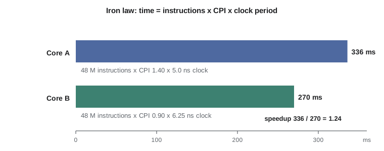
Maren has two candidate cores for the NS-5, both implementing the same RISC-V instruction set, so the classifier compiles to the same 48 million instructions per radar frame batch. Core A is a single-issue in-order core at 200 MHz with a measured CPI of 1.40. Core B is a dual-issue in-order core that closes timing at only 160 MHz but averages a CPI of 0.90. Which is faster, and by how much?
Show solution
- Core A takes 48 million instructions times 1.40 cycles, divided by 200 million cycles per second.
- \[ t_A = \frac{48 \times 10^{6} \times 1.40}{200 \times 10^{6}\ \text{Hz}} = 0.336\ \text{s}\]
- Core B takes 48 million instructions times 0.90 cycles, divided by 160 million cycles per second.
- \[ t_B = \frac{48 \times 10^{6} \times 0.90}{160 \times 10^{6}\ \text{Hz}} = 0.270\ \text{s}\]
- \[ \text{speedup} = \frac{t_A}{t_B} = \frac{0.336}{0.270} \approx 1.24\]
Answer: Core B is about 1.24 times as fast despite its 20 percent slower clock. Comparing clock rates alone would have chosen the wrong core.
Why MIPS and clock rate mislead
Because the iron law has three factors, any single-number rating that ignores two of them can mislead. Clock rate ignores CPI and instruction count, which is why a 3 GHz processor of one design can be slower than a 2.5 GHz processor of another. MIPS, millions of instructions per second, ignores instruction count: a compiler that emits more, simpler instructions raises MIPS while making the program slower, and two machines with different instruction sets cannot be compared by MIPS at all. Peak ratings, the throughput a machine reaches only if every unit is busy every cycle, describe a theoretical ceiling that real programs rarely approach. The only reliable measure is the execution time of real programs that resemble the intended workload.
Benchmarks
Since execution time depends on the program, architects agree on benchmark suites: collections of real programs, with defined inputs, that represent a class of workloads. Desktop and server processors are commonly compared with suites of integer and floating-point programs such as compilers, compression, simulation and scientific codes. Embedded processors have their own suites of small kernels such as filters, control loops and checksums, and machine learning hardware has suites that time training and inference on standard networks. A suite reports a summary, usually the geometric mean of each program's speedup relative to a reference machine, because the geometric mean gives the same ranking whichever machine is chosen as the reference.
Benchmarks can be gamed. A compiler can recognize a famous benchmark and apply an optimization that helps no other program; a vendor can report results on an unrealistic configuration. Good practice is to report the full configuration, to use the suite's rules, and above all to test the actual workload. For the NS-5, Maren insists that both candidate boards run Northway's own classifier on recorded radar frames from real roads. The suite numbers in the datasheets helped her shortlist the cores; only the classifier timing will decide.
Amdahl's law
An improvement to one part of a system helps only that part. If a fraction F of the execution time is sped up by a factor S and the rest is unchanged, the overall speedup is given by Amdahl's law.
The bound on the right is the sobering part: even an infinite speedup of the improved fraction cannot beat one over the unimproved fraction. If 40 percent of the time is spent in a filter kernel, making that kernel infinitely fast leaves 60 percent of the time untouched and caps the overall speedup at 1.67. Amdahl's law is the reason architects profile before they design: the biggest gains come from speeding up the common case, and a dramatic speedup of a rare case barely moves the total. The same law limits parallel processing, where F is the parallel fraction and S the number of processors, as lesson 10 shows.
Power and energy
Since the mid-2000s, power rather than transistor count has limited processor design. In CMOS logic, most power is dynamic, spent charging and discharging capacitance each time a signal switches. Dynamic power is proportional to the switched capacitance, the square of the supply voltage and the switching frequency, with an activity factor for the fraction of nodes that switch each cycle. Static or leakage power flows even when nothing switches and grows as transistors shrink and as temperature rises.
The square on voltage explains dynamic voltage and frequency scaling: lowering the clock allows a lower supply voltage, and energy per operation falls roughly with the square of voltage. It also explains the end of single-core clock scaling. Once supply voltages stopped falling with each process generation, raising the clock raised power density until chips could not be cooled, so designers turned to multiple cores and specialized units instead. For a battery or solar device such as the NS-5, energy per task often matters more than speed. A faster core that finishes and then sleeps can use less energy than a slower core that stays busy, a strategy sometimes called race to idle, but only if its power while running does not rise too much.
The program below applies the iron law and the power equation to Maren's two candidates, using capacitance and voltage figures from the vendors' models, and then asks what an 8-times faster vector unit for the filter kernel would buy. The capacitance values are illustrative.
# Iron law, Amdahl's law and dynamic power for two candidate NS-5 cores
cores = {
    "A: in-order, 1-issue": dict(f_mhz=200, cpi=1.40, instr=48.0e6, v=1.10, c_nf=0.30),
    "B: in-order, 2-issue": dict(f_mhz=160, cpi=0.90, instr=48.0e6, v=1.00, c_nf=0.45),
}
print("core                   time(ms)  MIPS   power(mW)  energy(mJ)")
res = {}
for name, k in cores.items():
    t = k["instr"] * k["cpi"] / (k["f_mhz"] * 1e6)          # iron law
    mips = k["instr"] / t / 1e6
    p = k["c_nf"] * 1e-9 * k["v"] ** 2 * k["f_mhz"] * 1e6   # P = C V^2 f
    e = p * t
    res[name] = (t, e)
    print(f"{name:22s} {t*1e3:8.1f} {mips:6.1f} {p*1e3:9.1f} {e*1e3:10.2f}")
(ta, ea), (tb, eb) = res.values()
print(f"speedup of B over A: {ta/tb:.2f}")
# Amdahl: an int8 vector unit speeds up the filter kernel, 40 % of B's time, by 8x
for frac, s in ((0.40, 8), (0.40, 1e9), (0.70, 8)):
print(f"fraction {frac:.2f}, kernel speedup {s if s < 1e6 else 'inf':>4}: overall {1/((1-frac)+frac/s):.2f}x")core time(ms) MIPS power(mW) energy(mJ) A: in-order, 1-issue 336.0 142.9 72.6 24.39 B: in-order, 2-issue 270.0 177.8 72.0 19.44 speedup of B over A: 1.24 fraction 0.40, kernel speedup 8: overall 1.54x fraction 0.40, kernel speedup inf: overall 1.67x fraction 0.70, kernel speedup 8: overall 2.58x
Core B is faster and, because it runs at a lower voltage, uses slightly less power while running, so it spends about 20 percent less energy per batch. The Amdahl lines show why Maren is cautious about the vector unit: an 8-times faster filter kernel gives about 1.5 times overall, and even an infinitely fast one gives only 1.67 times, unless the team can move more of the classifier, say 70 percent, onto it.
Cost, dependability and the design process
Performance and power are not the only constraints. The cost of a chip rises quickly with die area, because defects make large dies less likely to work; the cost of a system includes memory, packaging, boards and software effort. Dependability matters for devices bolted to poles for ten years: architects quantify it with mean time to failure and availability and improve it with redundancy and error-correcting codes. A quantitative design process states the workload, measures the current system, identifies the biggest contributors to time and energy, proposes changes, estimates their effect with models such as the iron law and Amdahl's law, and validates with simulation and measurement. The rest of this course supplies the models.
| Principle | What it says | Example in this course |
|---|---|---|
| Make the common case fast | Optimize what dominates time or energy | Caches exploit frequent reuse (lessons 7, 8) |
| Exploit parallelism | Overlap independent work at every level | Pipelines, superscalar issue, multicore (lessons 3, 5, 10) |
| Exploit locality | Recently used data and nearby data are likely to be used again | Cache and TLB design (lessons 7 to 9) |
| Specialize when general-purpose stalls | Dedicated hardware wins for narrow, heavy workloads | Vector units and accelerators (lesson 11) |
| Measure, do not guess | Base decisions on real workloads | The NS-5 trade study (lesson 12) |
Common mistakes
MistakeComparing processors by clock rate alone.
InsteadUse the iron law: execution time depends on instruction count, CPI and clock rate together.
MistakeUsing MIPS to compare machines with different instruction sets.
InsteadMIPS ignores instruction count. Compare execution times of the same real program.
MistakeExpecting a big speedup from accelerating a small part of the work.
InsteadApply Amdahl's law first. The unimproved fraction caps the overall gain at 1/(1 − F).
MistakeAssuming the faster core always uses more energy.
InsteadEnergy is power times time. A faster core at a lower voltage can use less energy per task.
MistakeAveraging speedups with the arithmetic mean.
InsteadBenchmark suites use the geometric mean of speedup ratios so the ranking does not depend on the reference machine.
Summary and key terms
- Execution time measures one task; throughput measures tasks per unit time.
- The iron law: CPU time = instruction count × CPI ÷ clock rate.
- CPI is a weighted average and is often reported as a base value plus stall components.
- Clock rate, MIPS and peak ratings mislead; real workloads and benchmark suites are the fair test.
- Amdahl's law limits overall speedup to 1/(1 − F) however fast the improved part becomes.
- Dynamic power scales with C V² f, so voltage scaling saves energy; leakage adds static power.
- Energy per task, cost and dependability are design constraints alongside speed.
- Execution time
- The time from the start to the end of one task; also called latency or response time.
- Throughput
- The number of tasks completed per unit of time.
- CPI
- Average clock cycles per instruction over a program.
- Iron law
- CPU time equals instruction count times CPI times clock period.
- Amdahl's law
- A formula giving overall speedup when only a fraction of execution is improved.
- Dynamic power
- Power spent switching capacitance, proportional to capacitance, voltage squared and frequency.
- Leakage power
- Power drawn by transistors even when they are not switching.
- Geometric mean
- The nth root of the product of n ratios, used to summarize benchmark speedups.
Practice problems
Work each problem on paper first, then reveal the answer to check.
A program runs 2 billion instructions at CPI 1.5 on a 2 GHz processor. What is its CPU time?
Show answer
2 × 10⁹ × 1.5 ÷ (2 × 10⁹ Hz) = 1.5 s.
Half of a program's time is in a loop that a new unit speeds up 10 times. What is the overall speedup?
Show answer
1 ÷ (0.5 + 0.5/10) = 1 ÷ 0.55 ≈ 1.82.
A designer lowers the supply voltage by 20 percent and the clock by 20 percent. Roughly how does dynamic power change?
Show answer
It scales by 0.8² × 0.8 ≈ 0.51, so it roughly halves.
Why can a compiler raise MIPS while slowing a program?
Show answer
By emitting more, simpler instructions with a low CPI: MIPS rises, but the extra instructions increase execution time.
Lesson quiz · 5 questions
Score 60% or more to complete this lesson.
Create a free account to save your progress, take quizzes and earn a certificate.