Differential and difference equations

Convolution tells you the output of an LTI system once you know its impulse response, but where does the impulse response come from? For circuits, mechanical systems and most digital filters, it comes from an equation that relates the output to the input and their rates of change. Continuous-time systems built from resistors, capacitors, inductors, masses and springs obey linear differential equations with constant coefficients. Digital filters obey linear difference equations, which are recipes for computing each new output from the latest input and a few earlier values. This lesson shows how to set up both kinds of equation, how to solve them, and how their solutions split into a part set by the system itself and a part set by the input.

A first-order circuit

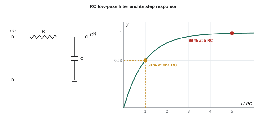
Return to the RC low-pass filter on the microphone channel. The input voltage x(t) drives a resistor R in series with a capacitor C, and the output y(t) is the capacitor voltage. The current through the resistor is (x − y)/R, and it all flows into the capacitor, whose current is C dy/dt. Setting the two equal gives the circuit's differential equation:

This is a first-order linear differential equation with constant coefficients. Linear means y and its derivatives appear only to the first power and are never multiplied together; constant coefficients means R and C do not change with time. Those two features are exactly what make the system linear and time-invariant, provided it starts at rest. Higher-order systems have higher derivatives: a series RLC circuit is second order, and the general Nth-order equation is

Natural and forced responses

The complete solution of a linear differential equation is the sum of two parts. The natural, or homogeneous, response y_h(t) solves the equation with the input set to zero. It depends only on the system and on its starting energy, such as the initial charge on the capacitor. The forced, or particular, response y_p(t) is any one solution that follows the input. For the RC circuit, setting x = 0 leaves RC dy/dt + y = 0, which an exponential e^(λt) solves if RCλ + 1 = 0. That equation in λ is the characteristic equation, and its root λ = −1/RC sets the natural response, Ae^(−t/RC). The constant A is found from the initial condition after the forced part has been added.

For a constant input x(t) = V applied at t = 0, try a constant forced response y_p = K. Substituting gives K = V. The complete response is y(t) = V + Ae^(−t/RC), and if the capacitor starts at y(0) = y₀, then A = y₀ − V:

The output starts at y₀ and moves exponentially toward V, covering 63 % of the remaining distance in each time constant. After five time constants it is within 1 % of V. The natural response dies away because its root is negative; a system whose characteristic roots all have negative real parts is stable, a link that lesson 11 makes precise.

Zero-input and zero-state responses

A second way to split the solution is often more useful for systems. The zero-input response is what the system does from its initial conditions with no input; the zero-state response is what the input produces with the system starting at rest. The complete response is their sum. The zero-state response is the one given by convolution with h(t), and it is the part that is linear in the input. The zero-input response is why a system with stored energy is not strictly linear in its input: doubling the input does not double the part caused by the initial charge. When engineers say a system is LTI, they mean its zero-state behaviour.

Second-order systems

A series RLC circuit, a mass on a spring with damping and a motor with load inertia all give second-order equations. Written in standard form with natural frequency ω_n and damping ratio ζ, the characteristic equation is λ² + 2ζω_nλ + ω_n² = 0, with roots

If ζ > 1 the roots are real and negative and the step response creeps up without overshoot, an overdamped system. If ζ = 1 it is critically damped, the fastest response with no overshoot. If ζ < 1 the roots are complex, and the natural response is a decaying sinusoid at the damped frequency ω_d = ω_n√(1 − ζ²): the system rings. A sensor mount on the pump that rings at its natural frequency is one reason Daniel sees bursts of noise in the tachometer signal. ELE-390 studies second-order systems in depth; here the point is that the roots of the characteristic equation tell you the shape of the natural response.

Difference equations

A digital filter computes each output from the current input and stored past values. The general linear constant-coefficient difference equation is

With a₀ = 1, it can be rearranged into a recursion that computes y[n] directly. If all the a coefficients after a₀ are zero, the output depends only on inputs, the impulse response has M + 1 terms and the filter is FIR; the moving averages of lesson 3 are examples. If any earlier output is fed back, the impulse response goes on forever and the filter is IIR.

Daniel's favourite IIR smoother is the exponential moving average:

Each new output moves a fraction α of the way from the previous output toward the new reading. It needs only one stored value instead of a whole window, which matters on a small microcontroller. Feeding in an impulse gives h[0] = α, h[1] = α(1 − α), h[2] = α(1 − α)², and in general h[n] = α(1 − α)ⁿu[n], a decaying geometric sequence. The filter is stable when |1 − α| < 1, and its DC gain is Σh[n] = 1, so steady readings pass unchanged. The characteristic root of the recursion is 1 − α, the discrete-time counterpart of λ: the closer it is to 1, the slower the response.

From a differential equation to a difference equation

A firmware engineer often has to implement an analog prototype as a digital filter. The simplest method replaces the derivative with a difference over one sample interval T. Using the backward difference dy/dt ≈ (y[n] − y[n − 1])/T in RC dy/dt + y = x gives

which is the exponential moving average with α = T/(RC + T). That is no coincidence: the exponential moving average is a digital RC filter. The approximation is good when T is much smaller than RC. Lesson 12 meets a better conversion, the bilinear transform, for when it is not.

Drawing a difference equation

Difference equations map directly onto block diagrams built from three parts: multipliers that scale a signal by a coefficient, adders, and unit delays that hold a value for one sample, drawn as a box labelled z⁻¹ for reasons that lesson 12 explains. The exponential moving average needs one delay that stores y[n − 1], one multiplier by 1 − α in the feedback path, one multiplier by α on the input and one adder. The diagram is also the program: each delay is a variable that keeps its value between readings, each multiplier is one multiplication, and the number of delays is the number of values the firmware must remember. That count, the order of the filter, sets its memory and its cost.

import math

RC, T = 0.16e-3, 0.02e-3            # time constant and sample interval, seconds
alpha = T / (RC + T)
y, out = 0.0, []
for n in range(60):                  # unit step input from n = 0
    y = (1 - alpha) * y + alpha * 1.0
    out.append(y)
for n in (8, 16, 40):
    exact = 1 - math.exp(-n * T / RC)
    print(f"t = {n*T*1e3:.2f} ms: digital {out[n-1]:.4f}  exact {exact:.4f}")

# Exponential moving average on tachometer readings every 50 ms
readings = [1200] * 5 + [1500] * 25
for a in (0.1, 0.3):
    y = readings[0]; hist = []
    for r in readings:
        y = (1 - a) * y + a * r
        hist.append(y)
    n63 = next(n for n in range(5, 30) if hist[n] >= 1200 + 0.63 * 300) - 4
    print(f"alpha = {a}: 63 % of the step after {n63} readings ({n63*50} ms)")

t = 0.16 ms: digital 0.6103  exact 0.6321
t = 0.32 ms: digital 0.8481  exact 0.8647
t = 0.80 ms: digital 0.9910  exact 0.9933
alpha = 0.1: 63 % of the step after 10 readings (500 ms)
alpha = 0.3: 63 % of the step after 3 readings (150 ms)

The digital filter lags the exact exponential by about two percentage points in the middle of the rise and catches up as both settle. The lag has a simple explanation: the backward-difference filter behaves like an RC filter whose time constant is RC + T instead of RC, one eighth longer here, so a smaller T would make the match closer. On the tachometer step, α = 0.1 reaches 63 % after 10 readings, as the worked example predicted, and α = 0.3 after 3 readings. A larger α follows changes faster but passes more noise, the same trade-off as the moving-average length in lesson 3.