The z-transform and digital filters

The Laplace transform is the natural language of circuits; the z-transform is its counterpart for sampled data and digital filters. It turns difference equations into algebra, explains why a unit delay is drawn as a box labelled z⁻¹, and lets an engineer judge the stability and frequency response of a digital filter by looking at its poles and zeros on a plane. This last lesson uses it to design the filter that finally removes the 60 Hz hum from Amara's microphone channel, to convert an analog filter into a digital one, and to pull together the whole signal chain of the accessible pedestrian signal.

Definition and region of convergence

The z-transform of a discrete-time signal x[n] is

where z is a complex variable. Writing z = re^(jΩ) shows the connection to the DTFT: on the unit circle, r = 1, the z-transform becomes X(e^(jΩ)), the frequency response or spectrum. Off the circle, the factor r^(−n) damps or amplifies the signal, just as e^(−σt) does in the Laplace transform, so the z-transform exists for signals, such as growing sequences, whose DTFT does not. The sum converges only for some z, the region of convergence. For a causal signal the ROC is the region outside a circle that passes through the outermost pole.

The most important pair is the geometric sequence. For x[n] = aⁿu[n],

Setting a = 1 gives the unit step, u[n] ↔ z/(z − 1), and the unit impulse transforms to 1. Damped and oscillating sequences follow by letting a be complex, just as damped sinusoids followed from complex exponentials in continuous time.

The delay property and transfer functions

Delaying a sequence by one sample multiplies its z-transform by z⁻¹: x[n − 1] ↔ z⁻¹X(z), for a signal at rest beforehand. That is why a unit delay in a block diagram is labelled z⁻¹, as in lesson 5. Applying the property term by term to a linear constant-coefficient difference equation turns it into an algebraic equation, and the ratio of output to input transforms is the transfer function:

The numerator coefficients b_k multiply delayed inputs and the denominator coefficients a_k multiply delayed outputs, so the transfer function can be read straight from the code and the code straight from the transfer function. The exponential moving average of lesson 5, y[n] = (1 − α)y[n − 1] + αx[n], has H(z) = α/(1 − (1 − α)z⁻¹) = αz/(z − (1 − α)): a zero at z = 0 and a pole at z = 1 − α.

Poles, zeros and stability in the z-plane

Factoring H(z) gives its zeros and poles, plotted on the z-plane with the unit circle drawn for reference. Each pole p contributes a term pⁿ to the impulse response. If |p| < 1 the term decays, if |p| = 1 it persists, and if |p| > 1 it grows. A causal digital filter is therefore stable if and only if all its poles lie strictly inside the unit circle. FIR filters have all their poles at z = 0 and are always stable; IIR filters must be checked. The exponential moving average has its pole at 1 − α, inside the circle for any α between 0 and 2, and the accumulator has its pole at z = 1, on the circle, which is why it is not BIBO stable.

The link to the s-plane comes from sampling. A continuous-time term e^(pt) sampled every T seconds becomes (e^(pT))ⁿ, so a pole at s = p maps to a pole at z = e^(pT). The left half of the s-plane maps to the inside of the unit circle, the imaginary axis maps to the circle itself, and the right half-plane maps outside. Stable analog filters become stable digital filters, and the further left an s-plane pole is, the closer to the origin its z-plane pole lands.

Reading the frequency response from the plane

Because the frequency response is H(z) on the unit circle, poles and zeros shape it geometrically. Imagine walking around the circle from Ω = 0 (z = 1, DC) to Ω = π (z = −1, the Nyquist frequency). The magnitude of H at each point is proportional to the product of the distances to the zeros divided by the product of the distances to the poles. A zero placed exactly on the circle at angle Ω₀ makes the response zero at that frequency. A pole placed just inside the circle at angle Ω₀ makes the response large near that frequency. The moving average's nulls from lesson 10 are zeros on the unit circle, and a resonator that emphasizes one frequency is a pole pair just inside it.

Designing a notch filter

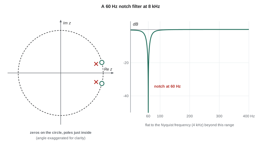
Amara's analog high-pass filter reduced the 60 Hz hum by only about 11 dB. A digital notch filter can remove it almost completely while leaving the rest of the band untouched. The recipe uses the geometry directly: place a pair of zeros on the unit circle at ±Ω₀, the hum frequency, to null it, and a pair of poles at the same angles but radius r slightly less than 1, so that away from Ω₀ each pole nearly cancels the effect of its neighbouring zero:

The closer r is to 1, the narrower the notch: its width is roughly (1 − r)f_s/π hertz. With r too close to 1, though, the filter takes a long time to settle, because its poles' terms rⁿ decay slowly, and rounding of the coefficients in fixed-point arithmetic can push the poles onto or outside the circle.

From analog to digital: the bilinear transform

Engineers often start from a proven analog design, such as a Butterworth filter, and convert it. Lesson 5's backward difference works only when the sampling interval is much shorter than the filter's time constants. The bilinear transform is better: it substitutes

into H(s). It maps the whole imaginary axis onto the unit circle exactly once, so a stable analog filter always gives a stable digital filter and there is no aliasing of the frequency response. The price is that the frequency axis is warped: analog frequency ω_a and digital frequency Ω are related by ω_a = (2/T)tan(Ω/2). To make a corner land at the right digital frequency, the designer prewarps it, choosing the analog corner from that formula before converting. Near DC the warping is negligible; near the Nyquist frequency it is severe.

The whole signal chain

Amara's final design for the accessible pedestrian signal uses nearly every idea in this course. The microphone feeds an analog high-pass filter that takes the edge off the 60 Hz hum and a fourth-order Butterworth anti-aliasing filter with a 2 kHz corner (lessons 8 and 9). The ADC samples at 8 kHz. In firmware, the hum notch removes what remains of the 60 Hz interference (this lesson). Every 50 ms, a 400-sample block is windowed and transformed with an FFT; bins from 300 Hz to 3 kHz, excluding a band around the 880 Hz tick, give the street noise level, and bin 44 gives the tick level (lesson 10). The noise level is smoothed by an exponential moving average (lesson 5) and fed to the volume loop, whose gain is limited for good damping (lesson 11). On the tachometer, a four-point moving average whose nulls cancel the pump's 5 Hz wobble cleans the speed reading (lessons 3 and 10). None of these steps is complicated on its own. What the course provides is the ability to predict, before writing a line of firmware, what each one will do.

import cmath, math

fs, f0, r = 8000.0, 60.0, 0.99
W0 = 2 * math.pi * f0 / fs
b = [1.0, -2 * math.cos(W0), 1.0]
a = [1.0, -2 * r * math.cos(W0), r * r]

def H(f):
    z = cmath.exp(1j * 2 * math.pi * f / fs)
    return (b[0] + b[1] / z + b[2] / z**2) / (a[0] + a[1] / z + a[2] / z**2)

for f in (0, 40, 50, 60, 70, 80, 880, 4000):
    g = abs(H(f))
    print(f"{f:5d} Hz: {20*math.log10(g) if g > 1e-12 else float('-inf'):8.1f} dB")

poles = [r * cmath.exp(1j * W0), r * cmath.exp(-1j * W0)]
print("pole radius", round(abs(poles[0]), 4), "-> stable" if all(abs(p) < 1 for p in poles) else "-> unstable")

# Filter one second of hum plus a quiet 880 Hz tone
x = [0.5 * math.cos(2 * math.pi * 60 * n / fs) + 0.05 * math.cos(2 * math.pi * 880 * n / fs)
     for n in range(8000)]
y = [0.0] * len(x)
for n in range(len(x)):
    y[n] = (b[0] * x[n] + (b[1] * x[n - 1] if n >= 1 else 0) + (b[2] * x[n - 2] if n >= 2 else 0)
            - (a[1] * y[n - 1] if n >= 1 else 0) - (a[2] * y[n - 2] if n >= 2 else 0))
def rms(v):
    return math.sqrt(sum(t * t for t in v) / len(v))
print(f"input RMS {rms(x[4000:]):.4f}, output RMS {rms(y[4000:]):.4f} (tone alone: {0.05/math.sqrt(2):.4f})")

    0 Hz:     -0.3 dB
   40 Hz:     -1.5 dB
   50 Hz:     -4.2 dB
   60 Hz:     -inf dB
   70 Hz:     -4.2 dB
   80 Hz:     -1.4 dB
  880 Hz:      0.1 dB
 4000 Hz:      0.1 dB
pole radius 0.99 -> stable
input RMS 0.3553, output RMS 0.0357 (tone alone: 0.0354)

The notch is infinitely deep at exactly 60 Hz, about 4 dB down 10 Hz either side and only about 1.5 dB down 20 Hz either side, which matches the estimated width of 25 Hz between the −3 dB points. At DC the loss is a third of a decibel, and at 880 Hz and 4 kHz the gain is within 0.1 dB of unity. The poles sit at radius 0.99, safely inside the circle. On the test signal, the hum dominates the input, but after the filter has settled the output RMS matches the quiet tone alone, so the hum has been removed and the tone kept. A deep notch built from five multiplications per sample is a small piece of code with a large effect, which is a fair summary of digital signal processing.