
CMP-229 · Lesson 1 of 12 · 37 min
Abstraction layers and computer performance
Every program you have written so far, from the Python of CMPUT-174 to the C of CMPUT-201, ran on hardware that you treated as a black box. You wrote x = y + z and something, somewhere, added two numbers. This course opens the box. Computer organization studies how a computer is built from the level of the instruction set downward: how numbers and text are stored as bits, what instructions a processor understands, how a compiler's output becomes a running program, how a processor is wired together from logic, and why memory is arranged as a hierarchy of fast small stores and slow large ones. The goal is not to make you a chip designer. It is to give you an accurate model of what your code actually does, so that you can write faster programs, read compiler output, debug problems that make no sense at the source level, and understand the security and reliability issues that start in the hardware.
This first lesson sets out the map. It describes the layers of abstraction that separate an application from transistors, the parts every computer shares, and the instruction set this course uses, RISC-V. It then gives you the most important quantitative tool in the subject: a precise way to measure and compare performance, including the performance equation, Amdahl's law and the power limits that shaped every processor of the last twenty years.
Layers of abstraction
A modern computer is too complex for anyone to hold in their head all at once, so it is built and understood as a stack of layers. Each layer offers a simpler interface to the layer above it and hides the details of the layer below. An application programmer sees a programming language and its libraries. The compiler translates that language into the instructions of a particular processor family. The instruction set architecture, or ISA, is the contract between software and hardware: the list of instructions, registers, data types and memory model that any processor in the family promises to implement. Below the ISA, the microarchitecture is one particular way of implementing that contract, with its own pipeline, caches and branch predictor. The microarchitecture is built from digital logic, logic is built from transistors, and transistors are physical devices etched into silicon.
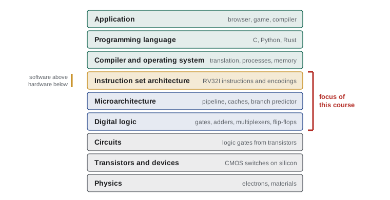
The ISA is the most important of these boundaries. Because it is a stable contract, the same compiled program runs on a cheap embedded RISC-V microcontroller and on a large server processor that implements the same instructions with ten times the speed. Intel and AMD have both sold x86-64 processors for two decades whose internal designs changed completely while old software kept working. Apple moved its laptops from x86-64 to the Arm ISA in 2020 and had to translate existing programs, which shows what changing the contract costs. When this course talks about organization, it means everything from the ISA down to the logic level; the layers below that belong to electrical and computer engineering.
Abstraction is not only a way of hiding detail; it is also a source of surprises. The C statement a[i] = 0 looks like one action, but on a real machine it may cost one cycle or hundreds depending on whether the memory holding a[i] is in a nearby cache. Integer arithmetic looks exact until a value overflows 32 bits. Floating point looks like real-number arithmetic until 0.1 + 0.2 fails to equal 0.3. Each of these effects comes from a lower layer leaking through, and each is explained in this course.
The stored-program computer and its five parts
Almost every computer in use today follows the stored-program design described in the 1940s by John von Neumann and his colleagues, building on ideas from Alan Turing and others: instructions are encoded as numbers and kept in the same memory as data. A processor repeatedly fetches the instruction at the address held in a special register, the program counter or PC, decodes it, executes it, and moves on to the next instruction. Because programs are data, a compiler can produce a program, a loader can copy it into memory, and an operating system can run many programs on one machine.
Textbooks traditionally divide a computer into five components. The datapath performs operations on data: it contains the registers and the arithmetic logic unit, or ALU. The control unit tells the datapath, memory and input/output devices what to do according to the instruction being executed; together, datapath and control form the processor, also called the central processing unit or CPU. Memory holds programs and data while they are running. Input devices bring information in, and output devices send it out. A phone has all five: its system-on-chip contains several processor cores and their caches, its memory chips are stacked beside it, the touch screen is both input and output, and the radio is an input/output device too.
| Component | Role | Where this course covers it |
|---|---|---|
| Datapath | Registers and the ALU that compute on data | Lessons 4, 9 and 10 |
| Control | Decodes instructions and directs the datapath | Lessons 9 and 10 |
| Memory | Holds instructions and data; organized as a hierarchy | Lessons 6, 11 and 12 |
| Input | Brings data in: keyboard, network, sensors | Lesson 12 |
| Output | Sends data out: display, network, actuators | Lesson 12 |
The ISA used in this course: RISC-V
This course uses the RISC-V instruction set, specifically its 32-bit base integer ISA, RV32I, with the multiply and divide extension M where it helps. RISC-V began at the University of California, Berkeley in 2010 and is now an open standard maintained by RISC-V International, a non-profit organization. Anyone can implement it without paying licence fees, which is why it is used in teaching, in research and in a fast-growing range of commercial products, from the small control processors inside storage drives and graphics cards to Linux-capable application processors. The base ISA is small enough to learn completely in a few weeks: RV32I has about forty instructions. Extensions add multiplication, atomic operations, floating point, compressed 16-bit instructions and vector operations, and profiles such as RVA23 bundle a set of extensions that operating systems can rely on.
RISC-V is a reduced instruction set computer, or RISC, design. RISC ISAs keep instructions simple and regular: every instruction is the same length, arithmetic works only on registers, and memory is accessed only by explicit load and store instructions. The alternative, complex instruction set computing or CISC, exemplified by x86-64, allows instructions of many lengths and lets arithmetic instructions read memory directly. Modern x86-64 processors translate their complex instructions into simple internal operations, so the distinction now matters more for instruction encoding and decoding than for speed. Arm, which powers nearly all phones and Apple's computers, is also a RISC design. The ideas you learn with RISC-V transfer directly to these machines, and lesson 8 compares the code compilers generate for RISC-V and x86-64.
Here is a taste of what you will be able to read by lesson 6: a short RISC-V assembly program that adds up an array of four numbers and prints the result. It was assembled with the LLVM assembler and run on the small RISC-V simulator used to produce every assembly output in this course, which follows the system-call conventions of RARS, a RISC-V simulator widely used in teaching. Do not worry about the details yet; notice the shape. Every line is one simple operation, the data lives in memory at labelled addresses, and a loop is just a backward branch.
    .data
arr:    .word 5, -3, 12, 8       # four 32-bit integers
msg:    .asciz "sum = "
    .text
    .globl main
main:
    la   t0, arr          # t0 = address of arr[0]
    li   t1, 4            # t1 = number of elements left
    li   a1, 0            # a1 = running sum
loop:
    lw   t2, 0(t0)        # t2 = *t0
    add  a1, a1, t2       # sum += t2
    addi t0, t0, 4        # advance to the next word
    addi t1, t1, -1       # one fewer element left
    bnez t1, loop         # repeat while elements remain
    la   a0, msg          # print the label
    li   a7, 4
    ecall
    mv   a0, a1           # print the sum
    li   a7, 1
    ecall
    li   a7, 10           # exit
ecallsum = 22 instructions executed: 33 ALU 22, loads 4, stores 0, branches 4 (3 taken), jumps 0, system 3
The statistics line is the first performance measurement in the course. The loop body has five instructions and runs four times, the set-up and printing add the rest, and you can check the total by hand. The counts by class matter because different kinds of instruction cost different amounts of time: loads go to memory, branches can disturb the pipeline, and lesson 10 shows how both affect speed.
What performance means
Saying one computer is faster than another needs a definition. For a single user, the important measure is usually response time, also called execution time or latency: how long one task takes from start to finish. For a data centre, the important measure is often throughput: how many tasks complete per unit time. The two are related but distinct. Adding more processor cores to a server raises throughput without making any single request finish sooner; replacing a processor with a faster one usually improves both.
When we compare execution times, we define performance as the reciprocal of execution time, so that bigger is better. If machine A runs a program in 10 seconds and machine B runs it in 15 seconds, then A is 15 / 10 = 1.5 times as fast as B. Phrases such as 50 per cent faster are ambiguous in everyday speech, so in this course \"A is n times as fast as B\" always means the ratio of execution times \(T_B / T_A = n\).
Execution time itself has more than one meaning. Wall-clock time includes everything: waiting for the disk, the network and other programs. CPU time counts only the time the processor spends running this program, and it divides into user CPU time, spent running the program's own instructions, and system CPU time, spent in the operating system on the program's behalf. The Unix time command reports all three, and the difference between them tells you whether a slow program is limited by computation or by waiting.
The performance equation
Processors run at a fixed clock rate, and every action takes a whole number of clock cycles. A clock rate of 3 GHz means \(3 \times 10^9\) cycles per second, so each clock cycle, or clock period, lasts \(1 / (3 \times 10^9)\) seconds, about 0.33 nanoseconds. The CPU time of a program is the number of clock cycles it needs multiplied by the length of one cycle. The number of cycles, in turn, is the number of instructions executed, the instruction count or IC, multiplied by the average number of clock cycles per instruction, or CPI. Putting these together gives the classic performance equation.
The equation is powerful because each factor is affected by different layers. The instruction count depends on the algorithm, the programming language, the compiler and the ISA. The CPI depends on the microarchitecture and on how well the program uses caches and branch prediction. The clock rate depends on the logic design and the manufacturing technology. Improving one factor often worsens another: a compiler that replaces several simple instructions with one complex one lowers the instruction count but may raise the CPI, and a deeper pipeline allows a faster clock but makes each stall more costly.
Worked problem
Comparing two processors
A program executes 2.0 × 10⁹ instructions. Processor A has a clock rate of 3.0 GHz and an average CPI of 1.6 for this program. Processor B runs the same machine code at 2.4 GHz with an average CPI of 1.1. Which processor is faster, and by how much?
Show solution
- CPU time on A = 2.0 × 10⁹ × 1.6 / (3.0 × 10⁹) = 1.067 s.
- CPU time on B = 2.0 × 10⁹ × 1.1 / (2.4 × 10⁹) = 0.917 s.
- B is faster despite its lower clock rate, because its CPI is much lower.
- Speedup of B over A = 1.067 / 0.917 = 1.16.
Answer: Processor B is about 1.16 times as fast as A for this program. Clock rate alone is a poor guide to performance.
The CPI in the equation is an average. Different instruction classes take different numbers of cycles, so the overall CPI is a weighted average over the program's instruction mix. Measuring the mix with hardware performance counters, which every modern processor provides, lets you calculate the CPI and see which class of instruction dominates the time.
# Average CPI from an instruction mix: CPI = sum(fraction_i * CPI_i)
mix = {           # class: (fraction of instructions, cycles each)
    'ALU':    (0.45, 1),
    'load':   (0.25, 3),
    'store':  (0.10, 2),
    'branch': (0.20, 2),
}
assert abs(sum(f for f, _ in mix.values()) - 1.0) < 1e-9
cpi = sum(f * c for f, c in mix.values())
print(f'average CPI = {cpi:.2f}')
for name, (f, c) in mix.items():
    share = f * c / cpi
    print(f'{name:>6}: {f:4.0%} of instructions, {share:5.1%} of cycles')

ic, clock = 5e9, 3.2e9            # instructions, cycles per second
print(f'CPU time = {ic * cpi / clock:.3f} s')average CPI = 1.80 ALU: 45% of instructions, 25.0% of cycles load: 25% of instructions, 41.7% of cycles store: 10% of instructions, 11.1% of cycles branch: 20% of instructions, 22.2% of cycles CPU time = 2.812 s
Loads are a quarter of the instructions but more than 40 per cent of the cycles. That pattern, a minority of instructions accounting for a majority of time, is common, and it tells you where to look for improvement: in this mix, making loads faster by improving the cache would pay off more than speeding up ALU operations.
Pitfalls: MIPS and peak numbers
Because the performance equation has three factors, any single number that captures only one of them misleads. Clock rate ignores CPI and instruction count. A once-popular measure, millions of instructions per second or MIPS, ignores instruction count: a processor that needs more, simpler instructions to do the same work can have a higher MIPS rating while running programs more slowly. Peak performance figures, such as the maximum floating-point operations per second a chip could perform if every unit were busy every cycle, describe a situation real programs rarely reach. The only trustworthy measure of performance is the time to run real programs.
For that reason the industry relies on benchmark suites: collections of real programs with standard inputs and rules for reporting results. The best known for processors are the SPEC CPU suites from the Standard Performance Evaluation Corporation. SPEC released SPEC CPU 2026 in May 2026, replacing the 2017 suite with new programs chosen to reflect current compilers, memory systems and workloads. Results are reported as ratios against a reference machine and summarized with the geometric mean, because the geometric mean of ratios gives the same ranking whichever machine is used as the reference.
Amdahl's law
Suppose you speed up one part of a program. How much faster does the whole program become? If the improved part originally took a fraction \(f\) of the execution time and you make it \(s\) times faster, the new time is \((1 - f) + f/s\) of the old time. The overall speedup is the reciprocal. This result, named after the computer architect Gene Amdahl, is the single most useful rule of thumb in performance work.
The law has a sobering consequence. Even if the improved part becomes infinitely fast, the overall speedup can never exceed \(1 / (1 - f)\). If 80 per cent of a program can run on many cores in parallel and 20 per cent must run on one core, no number of cores will make the program more than five times faster. The lesson for programmers is to make the common case fast: find where the time actually goes, which a profiler tells you, before optimizing anything.
def amdahl(f, s):
    """Overall speedup when a fraction f of the time is sped up s times."""
    return 1 / ((1 - f) + f / s)

print('fraction improved  s=2    s=10   s=100  s=inf')
for f in (0.5, 0.8, 0.9, 0.95, 0.99):
    row = [amdahl(f, s) for s in (2, 10, 100)] + [1 / (1 - f)]
print(f' {f:4.0%} ' + ' '.join(f'{x:5.2f}' for x in row))fraction improved s=2 s=10 s=100 s=inf
50% 1.33 1.82 1.98 2.00
80% 1.67 3.57 4.81 5.00
90% 1.82 5.26 9.17 10.00
95% 1.90 6.90 16.81 20.00
99% 1.98 9.17 50.25 100.00Worked problem
Deciding where to optimize
A program spends 60 per cent of its time in floating-point work and 25 per cent waiting for memory loads. Option 1 makes floating point 2 times faster. Option 2 makes memory loads 4 times faster. Which gives the larger overall speedup?
Show solution
- Option 1: 1 / (0.40 + 0.60/2) = 1 / 0.70 = 1.43.
- Option 2: 1 / (0.75 + 0.25/4) = 1 / 0.8125 = 1.23.
- Doing both: 1 / (0.15 + 0.60/2 + 0.25/4) = 1 / 0.5125 = 1.95.
Answer: Option 1 gives a speedup of about 1.43, more than option 2 at about 1.23, because it affects a larger fraction of the time. Doing both gives about 1.95.
The power wall and the turn to multicore
For decades, processors became faster mainly because their clock rates rose, from a few megahertz in the late 1970s to around 3 GHz by the mid-2000s. Then clock rates stopped climbing, and they have stayed in the range of roughly 3 to 6 GHz since. The reason is power. The dynamic power used by switching transistors is proportional to the capacitive load, the square of the supply voltage and the switching frequency. Halving the voltage cuts power by a factor of four, which is why each new manufacturing generation lowered voltages for many years, an effect known as Dennard scaling. Once voltages approached the level below which transistors leak too much current to switch reliably, further increases in frequency meant more heat than a chip could shed.
Designers responded by putting several processor cores on one chip instead of making one core faster. A modern laptop chip may have between eight and sixteen cores, some designed for speed and some for efficiency, alongside graphics and machine-learning accelerators. Transistor counts kept growing roughly as Gordon Moore predicted in 1965, doubling every two years or so, although the pace has slowed. The consequence for programmers is that more speed now comes mainly from parallelism, which software must be written to exploit, and from specialized hardware. Lesson 12 returns to parallel hardware; the CMPUT-379 and CMPUT-450 courses treat parallel software in depth.
# Dynamic power scales with C * V^2 * f. Compare a core run at full speed
# with two cores run at lower voltage and frequency.
def power(c, v, f):
    return c * v * v * f

base = power(1.0, 1.00, 3.0e9)
slow = power(1.0, 0.80, 2.0e9)       # 80% voltage, two-thirds frequency
print(f'one core at full speed : power 1.00, throughput 1.00')
print(f'one slower core        : power {slow / base:.2f}, throughput {2.0 / 3.0:.2f}')
print(f'two slower cores : power {2 * slow / base:.2f}, throughput {2 * 2.0 / 3.0:.2f}')one core at full speed : power 1.00, throughput 1.00 one slower core : power 0.43, throughput 0.67 two slower cores : power 0.85, throughput 1.33
Two cores at lower voltage and frequency deliver a third more throughput than one fast core while using about 15 per cent less power, provided the work can be split between them. That trade-off, multiplied across billions of devices and data centres whose electricity bills run to millions of dollars, explains why every processor you can buy today has multiple cores.
How this course is organized
The lessons follow the layers upward and then outward. Lessons 2 and 3 cover how integers, floating-point numbers and text are represented in bits. Lesson 4 builds the circuits that compute on those bits. Lessons 5 to 8 cover the RISC-V ISA and assembly programming: instructions and their encodings, control flow and memory, procedures and the stack, and how compilers, assemblers and linkers produce a running program. Lessons 9 and 10 design a processor that implements RV32I, first simply and then with a pipeline. Lessons 11 and 12 cover the memory hierarchy, virtual memory, input/output and parallelism, ending with a capstone that traces one program through every layer.
The prerequisites are modest. You need the programming and binary number basics of CMPUT-174, including the two's complement representation covered in its lesson 2, which lesson 2 here builds on. CMPUT-201's treatment of C, pointers and the stack is helpful for lessons 7 and 8 but is not required. ROB-200 covers digital electronics from an embedded-systems point of view; this course treats logic more abstractly, from the computer architect's side.
Common mistakes
MistakeComparing processors by clock rate alone.
InsteadUse CPU time = IC × CPI / clock rate; a lower-clocked processor with a lower CPI can be faster.
MistakeTreating MIPS or peak FLOPS as a measure of real performance.
InsteadMeasure the execution time of real programs, ideally a standard benchmark suite such as SPEC CPU 2026.
MistakeOptimizing the part of a program that is easiest to change rather than the part that takes the most time.
InsteadProfile first and apply Amdahl's law: the overall speedup is limited by the fraction you do not improve.
MistakeAssuming that doubling the cores halves the run time.
InsteadOnly the parallel fraction speeds up; with 20 per cent serial work, the speedup can never exceed 5.
MistakeThinking the ISA and the microarchitecture are the same thing.
InsteadThe ISA is the contract; many different microarchitectures can implement it with very different speeds.
Summary and key terms
- Computers are built as layers of abstraction; the instruction set architecture is the contract between software and hardware.
- Stored-program computers keep instructions and data in the same memory and repeatedly fetch, decode and execute instructions addressed by the PC.
- The five classic components are datapath, control, memory, input and output; datapath and control form the processor.
- This course uses RISC-V RV32I, an open RISC instruction set with fixed-length instructions and separate load and store instructions.
- Performance is the reciprocal of execution time; CPU time = instruction count × CPI × clock period.
- Amdahl's law limits the overall speedup to 1 / ((1 − f) + f/s), and to 1 / (1 − f) however large s becomes.
- Dynamic power is proportional to C × V² × f; the end of voltage scaling stopped clock rates rising and pushed designers to multicore chips.
- Instruction set architecture (ISA)
- The interface between software and hardware: the instructions, registers, data types and memory model a processor family implements.
- Microarchitecture
- A particular hardware implementation of an ISA, with its own pipeline, caches and other features.
- Program counter (PC)
- The register holding the address of the instruction being fetched.
- Datapath
- The part of the processor that holds and operates on data: registers, ALU and connections.
- RISC
- Reduced instruction set computer: an ISA style with simple, regular, fixed-length instructions and separate loads and stores.
- Response time
- The time to complete one task; also called execution time or latency.
- Throughput
- The amount of work completed per unit time.
- CPI
- Average clock cycles per instruction for a program on a given processor.
- Amdahl's law
- The rule that the overall speedup from improving part of a system is limited by the fraction of time the improvement affects.
- Dennard scaling
- The historical trend in which shrinking transistors allowed lower voltages, keeping power density constant as clock rates rose.
Practice problems
Work each problem on paper first, then reveal the answer to check.
A program executes 8 × 10⁹ instructions with an average CPI of 1.25 on a 2.5 GHz processor. What is its CPU time?
Show answer
8 × 10⁹ × 1.25 / (2.5 × 10⁹) = 4.0 seconds.
A new compiler reduces the instruction count by 20 per cent but raises the CPI from 1.25 to 1.4. Is the program faster?
Show answer
New time ∝ 0.8 × 1.4 = 1.12 compared with 1.25 before, so it is 1.25 / 1.12 ≈ 1.12 times as fast.
Machine A runs a benchmark in 12 s and machine B in 9 s. How many times as fast is B?
Show answer
12 / 9 ≈ 1.33.
Ninety per cent of a program can be parallelized. What is the maximum speedup with 8 cores and with unlimited cores?
Show answer
1 / (0.1 + 0.9/8) ≈ 4.71; with unlimited cores 1 / 0.1 = 10.
Name the five classic components of a computer.
Show answer
Datapath, control, memory, input and output.
Why is the ISA described as a contract?
Show answer
It specifies exactly what software can rely on, so any processor implementing it can run the same machine code.
If the supply voltage drops by 10 per cent and frequency is unchanged, by roughly what fraction does dynamic power fall?
Show answer
Power scales with V², so it becomes 0.81 of the original, a drop of about 19 per cent.
Why can MIPS rank two processors incorrectly?
Show answer
It ignores instruction count: a processor needing more simple instructions per task can have higher MIPS yet take longer.
Give one difference between RISC and CISC instruction sets.
Show answer
RISC instructions are fixed length and only loads and stores touch memory; CISC instructions vary in length and arithmetic can use memory operands.
Why does SPEC summarize results with the geometric mean?
Show answer
The geometric mean of performance ratios gives the same ranking regardless of which machine is the reference.
Lesson quiz · 5 questions
Score 60% or more to complete this lesson.
Create a free account to save your progress, take quizzes and earn a certificate.