
CMP-200 · Lesson 3 of 12 · 21 min
Arrays, memory layout and dynamic arrays
The array is the oldest and simplest data structure, and on real hardware it is very often the fastest. An array stores n elements of the same size in one contiguous block of memory. Because every element has the same size, the address of element i is a simple calculation, and the processor can fetch it in one step without looking at any other element. Almost every other structure in this course is built on arrays somewhere underneath: hash tables are arrays of slots, heaps are arrays read as trees, and even linked structures on a microcontroller are often carved out of a fixed array of nodes. This lesson looks at how arrays sit in memory, why that layout is so fast, and how a dynamic array grows without making every append expensive.
Maren gives Jonah a concrete job to anchor the lesson. The NS-4 keeps a running speed profile for each lane: the number of vehicles in each 5 km/h speed band from 0 to 200 km/h, reset every fifteen minutes. On the server, each node's reports are collected into a growing list of fifteen-minute summaries that analysts download and plot. The first is a fixed array on a microcontroller; the second is a dynamic array that grows as reports arrive. Between them they show nearly everything worth knowing about arrays.
Indexing: address arithmetic
If an array starts at address base and each element occupies s bytes, element i lives at address base + i·s. That one multiplication and addition is why reading or writing a[i] costs O(1), whatever the size of the array. In C, the expression a[i] is defined as exactly this calculation, and the compiler often turns it into a single load instruction with a scaled index. Indexing starts at 0 precisely so that the first element sits at the base address with no offset. The cost is that an array cannot grow in place: the memory just past its end may already belong to something else, so making it bigger means allocating a new block and copying.
Worked problem
Where is the element?
The NS-4 speed profile is an array of 40 unsigned 16-bit counters, one per 5 km/h band, starting at address 0x2000_1A40. Find the address of the counter for vehicles between 95 and 100 km/h, and the total size of the array.
Show solution
- Band i covers speeds from 5i to 5i + 5 km/h, so 95 to 100 km/h is band i = 95/5 = 19.
- Each counter is 16 bits, so s = 2 bytes.
- \[\text{address} = \text{0x20001A40} + 19 \times 2 = \text{0x20001A40} + 38\]
- In hexadecimal, 38 is 0x26.
- \[\text{address} = \text{0x20001A66}\]
- \[\text{size} = 40 \times 2 = 80 \text{ bytes}\]
Answer: The counter for 95 to 100 km/h is at 0x2000_1A66, and the whole profile occupies 80 bytes. Updating it for a passing vehicle is one division to find the band and one increment at a computed address: O(1).
Two-dimensional data, such as one speed profile per lane, is stored the same way. C lays a declaration like uint16_t profile[4][40] out in row-major order: all 40 counters for lane 0, then all 40 for lane 1, and so on, so element [lane][band] is at base + (lane·40 + band)·2. Fortran and some numerical libraries use column-major order instead. The difference matters for speed: a loop that walks along a row touches consecutive addresses, while a loop that walks down a column jumps 80 bytes each step. On a small microcontroller without a cache this costs nothing extra, but on a server processor the row-wise loop can be several times faster.
Why arrays are fast on real hardware
Lesson 1 mentioned the cache. A modern processor might execute several instructions per nanosecond, but a read from main memory takes on the order of 50 to 100 nanoseconds. To hide that gap, the processor keeps recently used memory in caches, small fast memories holding whole cache lines of 64 bytes. When a program reads element 0 of an array of 4-byte integers, the whole line holding elements 0 to 15 arrives at once, so the next 15 reads are nearly free. Better still, the hardware notices that the program is walking forward through memory and prefetches the following lines before they are asked for. This property, that nearby addresses are used close together in time, is called spatial locality, and arrays have as much of it as any structure can.
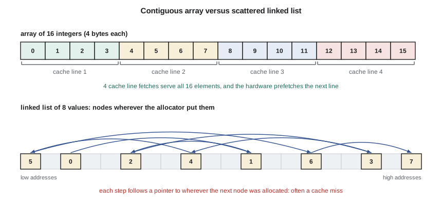
On the NS-4's microcontroller the story is simpler but related. It has no data cache, but its flash memory is slower than the processor, so a small instruction cache and a prefetch buffer serve the program code, and its RAM is single-cycle. Arrays still win there for different reasons: no pointer per element, so less memory; no pointer chasing, so fewer instructions; and predictable access times, which make worst-case timing easy to calculate. Direct memory access controllers, which copy data between peripherals and memory without the processor, also work naturally with contiguous arrays. The radar samples arrive by DMA into an array, never into a linked structure.
Fixed-size arrays and their limits
A fixed-size array is ideal when the maximum size is known in advance, as it is for the speed profile. It has no overhead at all, and every operation by index is O(1). Its weakness is anything that changes the arrangement. Inserting a new element at position i means shifting every element from i to the end one place to the right, which costs O(n − i) moves, O(n) in the worst case. Deleting from the middle shifts the rest left by the same amount. Searching an unsorted array for a value is O(n). And if the array fills up, a fixed array simply cannot take more. Embedded designers live with these limits deliberately, sizing each array for the worst case they will ever see and testing what happens at the boundary.
Dynamic arrays
On the server, the number of fifteen-minute summaries for a node grows without a known limit, and the analysts want fast access by index to plot any day. The structure for this is the dynamic array, called list in Python, vector in C++ and ArrayList in Java. It keeps an underlying fixed array, the backing store, that is usually larger than the number of elements in use. Two numbers describe it: the size, how many elements are in use, and the capacity, how many the backing store can hold. Appending when size < capacity simply writes the new element at position size and increments size: O(1). When size reaches capacity, the dynamic array allocates a new, larger backing store, copies all the elements across, frees the old one and then appends.
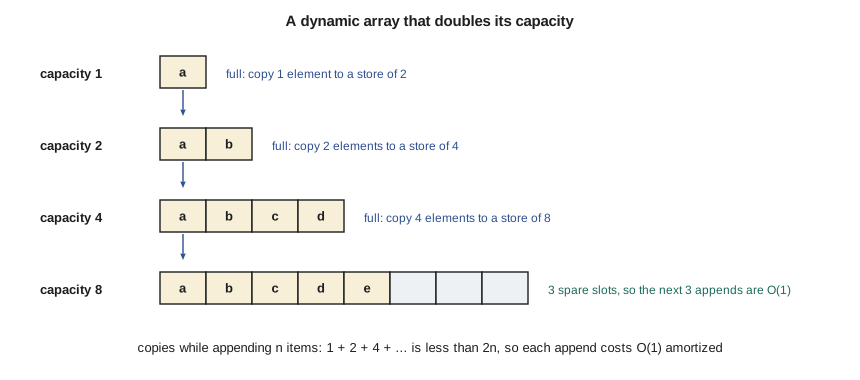
The interesting question is how much larger the new backing store should be. If it grew by a constant amount, say 10 slots each time, then appending n elements would trigger about n/10 resizes, and the k-th resize would copy about 10k elements. The total copying would be about 10·(1 + 2 + … + n/10) ≈ n²/20, which is O(n²): quadratic, just like the duplicate check in lesson 2. If instead the capacity doubles at each resize, the copies made while appending n elements are 1 + 2 + 4 + … up to n, which sums to less than 2n. Spread over n appends, that is fewer than two copies per append on average. So appending to a doubling dynamic array costs O(1) amortized, even though an individual append that triggers a resize costs O(n).
# Count element copies while appending n items to a dynamic array
def total_copies(n, grow):
    size, cap, copies = 0, 1, 0
    for _ in range(n):
        if size == cap:
            copies += size          # copy every element into the new store
            cap = grow(cap)
        size += 1
    return copies

for n in (1_000, 10_000, 100_000):
    d = total_copies(n, lambda c: 2 * c)
    a = total_copies(n, lambda c: c + 10)
    print(f"n = {n:>7,}: doubling {d:>9,} copies ({d / n:.2f} per append), "
f"add-10 {a:>13,} copies ({a / n:,.0f} per append)")n = 1,000: doubling 1,023 copies (1.02 per append), add-10 49,600 copies (50 per append) n = 10,000: doubling 16,383 copies (1.64 per append), add-10 4,996,000 copies (500 per append) n = 100,000: doubling 131,071 copies (1.31 per append), add-10 499,960,000 copies (5,000 per append)
The output makes the difference concrete. With doubling, the number of copies per append stays below 2 however large n gets. With a fixed increment of 10, the copies per append grow in proportion to n, reaching thousands per append at n = 100,000. Real implementations usually grow by a factor between 1.5 and 2. A smaller factor wastes less memory, at most a third of the backing store empty instead of half, at the price of slightly more copying; CPython's list grows by roughly one eighth plus a constant, which still gives amortized O(1) appends because the growth is proportional to the current size. The proportional growth is the essential part.
Amortized cost is a statement about the total, not about each operation. Most appends are cheap, but one in a while is expensive: appending the millionth element to a doubling array copies a million elements at once. On a server that pause is usually harmless. In a real-time loop it is not, which is one more reason the NS-4 firmware never grows arrays at run time. When a server process must avoid pauses, it can reserve capacity in advance, for example with reserve() on a C++ vector, or use a structure whose growth is incremental, such as a list of fixed-size chunks.
/* A minimal growable array of 32-bit values (server-side C) */
#include <stdlib.h>
#include <stdint.h>

typedef struct { uint32_t *data; size_t size, cap; } vec_t;

int vec_push(vec_t *v, uint32_t x)
{
    if (v->size == v->cap) {
        size_t ncap = v->cap ? 2 * v->cap : 8;          /* double the capacity */
        uint32_t *p = realloc(v->data, ncap * sizeof *p);
        if (p == NULL) return -1;                         /* old block still valid */
        v->data = p;
        v->cap = ncap;
    }
    v->data[v->size++] = x;
    return 0;
}
The C listing shows two details that Python hides. First, realloc can fail, and if it does the old block is still valid, so the code assigns the result to a temporary pointer and checks it before overwriting v->data; writing v->data = realloc(v->data, …) directly would leak the old block on failure. Second, any pointer into the old backing store becomes invalid after a resize, because the data may have moved. Code that saved the address of element 5 and then appended an element may now be reading freed memory. The same rule applies to C++ iterators and to references into a vector. In Python the list manages its own memory, so you cannot see this hazard, but you can still see its cost.
Deleting and shrinking
Removing the last element of a dynamic array is O(1): decrement the size. Removing from the front or middle costs O(n) because the remaining elements shift. Some implementations also shrink the backing store when it becomes mostly empty, to return memory. The rule must be chosen carefully: if an array doubles when full and halves as soon as it is half full, a sequence that alternately appends and removes at the boundary triggers a resize every time, and each costs O(n). The standard fix is to halve only when the array falls to a quarter full, which keeps the amortized cost of both appends and removals at O(1).
| Operation | Fixed array | Dynamic array |
|---|---|---|
| Read or write a[i] | O(1) | O(1) |
| Append at the end | O(1) until full, then impossible | O(1) amortized, O(n) worst case |
| Remove from the end | O(1) | O(1) amortized |
| Insert or delete at position i | O(n − i) | O(n − i) |
| Search for a value (unsorted) | O(n) | O(n) |
| Memory overhead | None | Spare capacity, up to about half the store |
Common mistakes
MistakeGrowing a dynamic array by a fixed number of slots each time it fills.
InsteadGrow by a constant factor, such as 1.5 or 2, so that total copying stays proportional to n and appends are O(1) amortized.
MistakeKeeping a pointer or reference to an element and then appending to the array.
InsteadA resize may move the data. Re-read the address after any operation that can grow the array, or store indexes instead of pointers.
MistakeWriting p = realloc(p, n) in C.
InsteadAssign to a temporary, check for NULL, and only then replace the original pointer, so a failed allocation does not leak the old block.
MistakeRemoving items from the front of a large Python list in a loop.
InsteadEach removal shifts every remaining element, making the loop O(n²). Use collections.deque or an index that moves forward.
MistakeWalking a two-dimensional array column by column in a performance-critical loop.
InsteadIn C's row-major layout, loop over the last index innermost so that memory is accessed consecutively.
Summary and key terms
- An array stores equal-sized elements contiguously, so element i is at base + i·s and indexing costs O(1).
- Contiguous storage gives spatial locality, so arrays make excellent use of caches and prefetching.
- Inserting or deleting in the middle shifts elements and costs O(n); a fixed array cannot grow.
- A dynamic array keeps spare capacity and grows by a constant factor, giving O(1) amortized appends with occasional O(n) resizes.
- Resizes move data, invalidating pointers into the array, and cause pauses that real-time code must avoid.
- Array
- A contiguous block of memory holding elements of equal size, accessed by index.
- Row-major order
- Storing a two-dimensional array row by row, so elements of a row are adjacent in memory.
- Spatial locality
- The tendency of a program to use addresses close to ones it has just used.
- Dynamic array
- An array that grows by allocating a larger backing store and copying its elements when full.
- Capacity
- The number of elements a dynamic array's backing store can hold before it must grow.
- Amortized O(1)
- Constant cost per operation on average over any long sequence, even if some single operations cost more.
Practice problems
Work each problem on paper first, then reveal the answer to check.
An array of 8-byte doubles starts at address 1000. What is the address of element 25?
Show answer
1000 + 25 × 8 = 1200.
For uint16_t m[10][30] in C, how many bytes separate m[2][5] from m[3][5]?
Show answer
One row of 30 elements of 2 bytes: 60 bytes.
A doubling dynamic array starts at capacity 1. How many element copies are made while appending 64 elements?
Show answer
1 + 2 + 4 + 8 + 16 + 32 = 63 copies.
Why does halving a dynamic array as soon as it is half full cause trouble?
Show answer
Alternating appends and removals at the boundary would trigger a resize on every operation, each costing O(n).
Inserting at the front of a dynamic array of 10,000 elements moves how many elements?
Show answer
All 10,000 shift one place: O(n).
Lesson quiz · 5 questions
Score 60% or more to complete this lesson.
Create a free account to save your progress, take quizzes and earn a certificate.