
CMP-200 · Lesson 10 of 12 · 21 min
Hash tables
A hash table stores key and value pairs and finds the value for a given key in constant time on average, however many pairs it holds. It achieves this with a simple idea: instead of searching for the key, compute where it should be. A hash function turns the key into an integer, and that integer, reduced to the size of an underlying array, picks the slot where the pair is stored. Looking a key up later repeats the same calculation and goes straight to the same slot. Hash tables are the most heavily used data structure in modern software: Python's dict and set, JavaScript objects, the symbol tables of compilers and assemblers, database hash joins, network routers' flow tables, caches of every kind, and the duplicate check that rescued Jonah's server in lesson 2 all depend on them.
Northway's server uses hash tables in two places Jonah now owns. The first maps each node's serial number to its configuration and status record, about 800 entries consulted on every upload. The second is the set of record identifiers already stored for the day, used to reject duplicate uploads, which reaches 40,000 entries per busy node. On the NS-4 itself, a small hash table maps the 16-bit identifiers of vehicles' toll transponders, read by an optional radio module on some highway installations, to the time each was last seen, so that a vehicle seen at two nodes can be matched for travel-time estimates. That table must live in a fixed 8 KB block of RAM and never stall the main loop.
Hash functions
A hash function maps a key of any type to an integer called its hash value or hash code. To be useful it must be deterministic, always giving the same hash for the same key, and fast, and it should spread typical keys evenly over the range, so that different keys rarely land in the same slot. The slot index is then the hash reduced to the table size m, usually as hash mod m, or, when m is a power of two, by keeping the low bits with hash & (m − 1). A poor hash function is the commonest cause of a slow hash table. Taking only the last few digits of a serial number, for instance, fails badly if Northway assigns serial numbers in blocks that all end in the same digits.
For integer keys, a simple and effective hash multiplies the key by a large odd constant and keeps the high bits of the product, which mixes every bit of the key into the result; this is called multiplicative or Fibonacci hashing when the constant is derived from the golden ratio. For strings, a hash combines the characters one at a time, for example h = h × 31 + c for each character code c, as Java's String.hashCode does. Well-tested general-purpose functions such as FNV-1a, MurmurHash and SipHash do this mixing more thoroughly. Python uses SipHash for strings, with a random key chosen when the interpreter starts, so that an attacker who sends specially chosen keys to a web server cannot force all of them into the same slot; that attack, called hash flooding, once let a few kilobytes of crafted input tie up a server's processor for minutes.
# FNV-1a 32-bit hash of node serial numbers, and how evenly they spread over 16 slots
def fnv1a_32(s):
    h = 0x811C9DC5
    for b in s.encode():
        h ^= b
        h = (h * 0x01000193) & 0xFFFFFFFF
    return h

def last_digit(s):                   # a poor hash: only the final character
    return ord(s[-1])

serials = [f"NS4-{block:02d}-{unit:03d}0" for block in range(4) for unit in range(60)]

for name, fn in (("last digit", last_digit), ("FNV-1a", fnv1a_32)):
    counts = [0] * 16
    for s in serials:
        counts[fn(s) % 16] += 1
print(f"{name:>10}: slot counts {counts} max {max(counts)}")last digit: slot counts [240, 0, 0, 0, 0, 0, 0, 0, 0, 0, 0, 0, 0, 0, 0, 0] max 240
FNV-1a: slot counts [17, 12, 17, 14, 19, 12, 19, 10, 12, 17, 14, 17, 12, 19, 10, 19] max 19The experiment hashes 240 serial numbers that all happen to end in zero, as Northway's do because the last digit is reserved for a revision code. The poor hash sends every one of them to the same slot, turning the table into a linked list. FNV-1a spreads them close to the ideal of 15 per slot. Real data is full of patterns like this, which is why a hash function must mix all the bits of the key and not just use the convenient ones.
Collisions and load factor
Two different keys that land in the same slot collide. Collisions are unavoidable: there are far more possible keys than slots, and by the birthday paradox they start surprisingly early. With 365 slots and random keys, the chance of at least one collision passes 50 percent at just 23 keys. A hash table's design is therefore mostly about handling collisions. The key parameter is the load factor α = n/m, the number of stored entries divided by the number of slots. The expected cost of operations depends on α, not on n itself, so a table that grows its slot array to keep α bounded, by doubling and rehashing every entry into the new array as a dynamic array does, keeps operations O(1) on average and its growth costs O(1) amortized.
Separate chaining
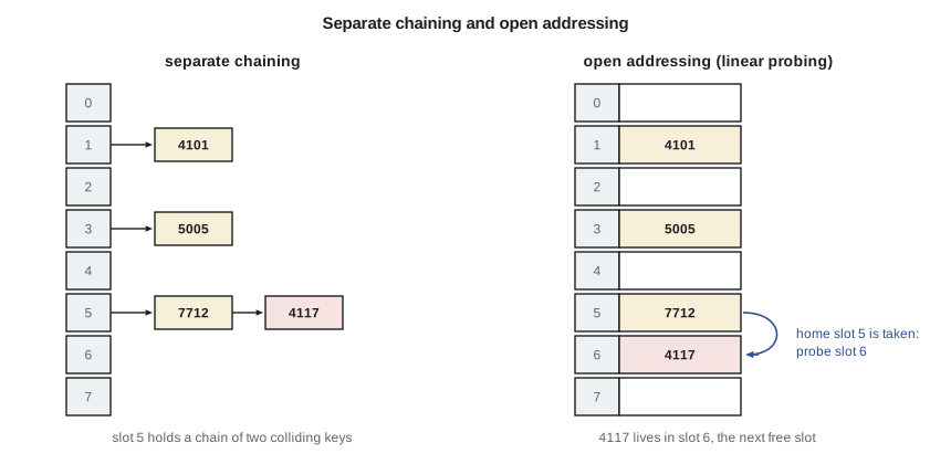
The simplest collision strategy is separate chaining: each slot holds a pointer to a linked list, called a chain or bucket, of all the entries whose keys hash to that slot. Inserting puts the new entry at the front of its chain, after checking that the key is not already present. Looking up a key hashes it, then walks that one chain comparing keys. With a good hash function, the expected chain length is α, so an unsuccessful search examines about α entries and a successful one about 1 + α/2. Chaining degrades gracefully as α grows past 1, and deleting is easy, just unlink the node, but every entry costs an extra pointer and the chains scatter entries across memory. Java's HashMap uses chaining and converts a long chain into a small balanced tree when it exceeds eight entries, which caps the worst case at O(log n) even under attack.
Open addressing
Open addressing stores every entry directly in the slot array, with no chains. When a key's home slot is occupied, the table probes a sequence of other slots until it finds an empty one. The simplest sequence is linear probing: try slots h, h + 1, h + 2 and so on, wrapping around the end. Lookup follows the same sequence until it finds the key or reaches an empty slot, which proves the key is absent. Linear probing is very cache-friendly, because the probes touch consecutive slots, and it needs no pointers, so modern high-performance tables such as Google's Swiss tables and Rust's standard HashMap use open addressing. Its weakness is clustering: occupied slots tend to form runs, and a new key landing anywhere in a run must walk to its end, which lengthens the run further. The expected cost grows sharply as α approaches 1.
Worked problem
Choosing a load factor for linear probing
The NS-4 transponder table uses linear probing. Using Knuth's approximations, estimate the expected probes for an unsuccessful search, the common case when a vehicle is seen for the first time, at load factors 0.5, 0.75 and 0.9. If each slot holds a 2-byte identifier and a 4-byte time and the table must hold up to 900 vehicles, how many slots should the 8 KB block provide?
Show solution
- Apply the unsuccessful-search formula.
- \[\alpha = 0.5: \tfrac12\big(1 + 1/0.25\big) = 2.5 \text{ probes}\]
- \[\alpha = 0.75: \tfrac12\big(1 + 1/0.0625\big) = 8.5 \text{ probes}\]
- \[\alpha = 0.9: \tfrac12\big(1 + 1/0.01\big) = 50.5 \text{ probes}\]
- Keeping α at or below about 0.7 at the maximum of 900 vehicles needs at least 900/0.7 ≈ 1,286 slots; a power of two lets the index be computed with a bitwise AND, so 2,048 slots, giving α ≈ 0.44 when full.
- \[2048 \times (2 + 4) = 12\,288 \text{ bytes} > 8\,192\]
- That is too large. 1,024 slots use 6,144 bytes and fit, but give α ≈ 0.88 when full, so the design caps the table at about 700 live entries (α ≈ 0.68) and evicts the oldest sightings beyond that.
Answer: About 2.5, 8.5 and 50.5 probes. The team uses 1,024 slots (6 KB) with an eviction rule that keeps the load factor below 0.7, accepting that very old sightings are forgotten during the busiest hour.
Deletion is the awkward operation in open addressing. Simply emptying a slot would break the probe chains of keys that were placed beyond it, so a later lookup would stop at the hole and wrongly report them missing. The usual fix is a tombstone, a marker meaning deleted, which lookups skip over and insertions may reuse. Tombstones accumulate, so the table is rebuilt from time to time. Linear probing also allows a cleverer delete, backward shift deletion, which moves later entries of the run back into the hole and avoids tombstones entirely; the NS-4 uses it so that the table never needs a rebuild in the field.
# Linear probing with backward-shift deletion, for 16-bit transponder ids
EMPTY = None

class ProbeTable:
    def __init__(self, m=16):
        self.m, self.keys, self.vals, self.n = m, [EMPTY] * m, [None] * m, 0

    def _home(self, k):
        return (k * 40503) & 0xFFFF & (self.m - 1)   # multiplicative hash, m a power of 2

    def put(self, k, v):
        i = self._home(k)
        while self.keys[i] is not EMPTY and self.keys[i] != k:
            i = (i + 1) & (self.m - 1)
        if self.keys[i] is EMPTY:
            self.n += 1
        self.keys[i], self.vals[i] = k, v

    def get(self, k):
        i, probes = self._home(k), 1
        while self.keys[i] is not EMPTY:
            if self.keys[i] == k:
                return self.vals[i], probes
            i, probes = (i + 1) & (self.m - 1), probes + 1
        return None, probes

    def delete(self, k):
        i = self._home(k)
        while self.keys[i] is not EMPTY and self.keys[i] != k:
            i = (i + 1) & (self.m - 1)
        if self.keys[i] is EMPTY:
            return False
        j = i
        while True:                                 # shift later run members back
            j = (j + 1) & (self.m - 1)
            if self.keys[j] is EMPTY:
                break
            home = self._home(self.keys[j])
            # move keys[j] into the hole at i if its home is not between i and j cyclically
            if (j > i and (home <= i or home > j)) or (j < i and (home <= i and home > j)):
                self.keys[i], self.vals[i] = self.keys[j], self.vals[j]
                i = j
        self.keys[i], self.vals[i] = EMPTY, None
        self.n -= 1
        return True

t = ProbeTable(16)
for tid, ts in ((4101, 30_005), (4117, 30_010), (5005, 30_012), (4133, 30_020), (7712, 30_021)):
    t.put(tid, ts)
print("slots:", t.keys)
t.delete(4117)
print("after deleting 4117:", t.keys)
for tid in (4101, 4133, 4117):
    print(f"get {tid}: {t.get(tid)}")
print(f"load factor {t.n / t.m:.2f}")slots: [7712, None, None, 4101, 4117, 4133, None, None, None, None, None, 5005, None, None, None, None] after deleting 4117: [7712, None, None, 4101, 4133, None, None, None, None, None, None, 5005, None, None, None, None] get 4101: (30005, 1) get 4133: (30020, 2) get 4117: (None, 3) load factor 0.25
Hash tables in practice
Several practical points decide whether a hash table performs as the theory promises. Keys must not change while they are in the table: if a key's hash changes, the entry is stranded in the wrong slot. This is why Python allows only immutable objects, such as strings, numbers and tuples of them, as dictionary keys. Equality and hashing must agree: two keys that compare equal must have the same hash, so if you define a custom key type you must define both together. Resizing must be planned: a table that doubles when α passes a threshold occasionally pauses to rehash every entry, which is harmless on a server but not acceptable in an interrupt handler, so firmware tables are sized in advance or rehash incrementally. Finally, iteration order is not sorted. Python dicts happen to remember insertion order, a guarantee since Python 3.7, but a hash table never keeps keys in sorted order, so range queries need the search trees of lesson 8.
| Operation | Hash table (average) | Hash table (worst) | Balanced BST | Sorted array |
|---|---|---|---|---|
| Insert | O(1) | O(n) | O(log n) | O(n) |
| Lookup by key | O(1) | O(n) | O(log n) | O(log n) |
| Delete | O(1) | O(n) | O(log n) | O(n) |
| Range query | O(n) | O(n) | O(log n + k) | O(log n + k) |
| Minimum or successor | O(n) | O(n) | O(log n) | O(1) or O(log n) |
| Iterate in key order | Requires sorting | Requires sorting | O(n) | O(n) |
Common mistakes
MistakeUsing a hash function that looks only at part of the key, such as the last digits.
InsteadUse a well-tested function such as FNV-1a, MurmurHash or SipHash that mixes every bit of the key.
MistakeLetting the load factor of an open-addressing table approach 1.
InsteadProbe counts explode near α = 1; resize, or cap entries, to keep α below about 0.7.
MistakeEmptying a slot to delete from an open-addressing table.
InsteadUse tombstones or backward-shift deletion so that later keys in the probe run remain reachable.
MistakeChanging a key, or defining equality without a matching hash, for a key stored in a table.
InsteadKeys must be immutable while stored, and equal keys must have equal hashes.
MistakeUsing a hash table when the program needs keys in order or range queries.
InsteadHash tables do not keep order; use a balanced search tree or a sorted structure.
Summary and key terms
- A hash table computes a slot from the key's hash, giving O(1) average-time insert, lookup and delete.
- A good hash function is deterministic, fast and spreads typical keys evenly; randomized hashing defends against hash flooding.
- Collisions are unavoidable; their cost depends on the load factor α = n/m, kept bounded by resizing.
- Separate chaining keeps a list per slot; open addressing probes other slots and is more cache-friendly but sensitive to high load.
- Hash tables need immutable keys, consistent equality and hashing, and do not support ordered or range queries.
- Hash function
- A function that maps a key to an integer used to choose a slot.
- Collision
- Two different keys mapping to the same slot.
- Load factor
- The ratio α = n/m of stored entries to slots.
- Separate chaining
- Resolving collisions by keeping a linked list of entries in each slot.
- Open addressing
- Resolving collisions by probing other slots of the array until a free one is found.
- Linear probing
- Open addressing that tries consecutive slots after the home slot.
- Tombstone
- A marker left in an open-addressing slot to show that an entry was deleted.
Practice problems
Work each problem on paper first, then reveal the answer to check.
A chained hash table has 1,000 slots and 2,500 entries. What is the expected number of entries examined in an unsuccessful search?
Show answer
α = 2.5, so about 2.5 entries.
For linear probing at α = 0.8, estimate the expected probes for an unsuccessful search.
Show answer
½(1 + 1/0.04) = 13 probes.
Why is m usually a power of two in tables that use hash & (m − 1)?
Show answer
Only then does the bitwise AND give the remainder modulo m, and it is cheaper than division.
Why can't a Python list be used as a dictionary key?
Show answer
Lists are mutable, so their hash could change while stored; Python only allows hashable, immutable keys.
A table of 512 slots must hold up to 400 entries with linear probing. Is that a good design?
Show answer
No: α ≈ 0.78 when full, giving long probe runs; use 1,024 slots or cap the entries.
Lesson quiz · 5 questions
Score 60% or more to complete this lesson.
Create a free account to save your progress, take quizzes and earn a certificate.