
CMP-200 · Lesson 1 of 12 · 24 min
Data structures, abstract data types and the cost of an operation
Every program that does anything useful stores data and looks it up again. A thermostat keeps the last hour of temperature readings, a web server keeps a table of logged-in users, and a compiler keeps the names of every variable it has seen. How that data is arranged in memory decides how fast the program runs, how much memory it needs and, on small embedded devices, whether it fits at all. A data structure is a particular way of arranging data so that certain operations are cheap. An algorithm is a finite, precise sequence of steps that solves a problem, usually by working on data held in one or more data structures. This course is about choosing, building and measuring both, with the eye of a computer engineer who has to make them run on real hardware.
In a CEAB-accredited Canadian computer engineering program, Data Structures and Algorithms usually comes in the fall of second year, right after a first programming course such as ENCM-100. It is the foundation for nearly everything that follows: operating systems manage processes in queues and memory in free lists, compilers use trees and hash tables, networks route packets with graph algorithms, and embedded firmware lives or dies by how carefully it uses a few kilobytes of RAM. Later, CMP-301 Algorithm Design builds on it with greedy algorithms, dynamic programming and hard problems, and CMPUT-204 Algorithms I covers the mathematics of sorting and graph algorithms in more depth.
The examples follow Northway Sensing, an invented company in Kingston, Ontario that makes roadside traffic counters for cities and provincial highway departments. Its NS-4 counter node sits in a weatherproof box beside the road, reads a radar sensor and two inductive loops cut into the pavement, classifies each passing vehicle, and uploads counts to a server every few minutes over a cellular modem. The node runs on a 32-bit microcontroller with 256 KB of flash and 64 KB of RAM. Maren Holt, P.Eng., leads the firmware team. Jonah Abara, a second-year computer engineering co-op student, has just joined her, and each lesson follows a problem she hands him, on the node or on the server that collects its data.
What a data structure is
Think of the vehicle records the NS-4 produces. Each record holds a timestamp, a lane number, a speed and a vehicle class, about 12 bytes in a compact form. The firmware needs to add new records as vehicles pass, remove the oldest records once they have been uploaded, and occasionally answer questions such as how many trucks went by in the last fifteen minutes. The server, in contrast, holds millions of records from hundreds of nodes and must answer queries such as which nodes have reported unusual speeds today. The same records, the same fields, but completely different arrangements make sense in the two places. On the node, a fixed-size circular buffer is ideal: adding and removing are instant, and the memory never grows. On the server, indexes built from trees and hash tables let a query skip almost all of the data.
A data structure therefore has two sides. One side is the layout: where each piece of data sits in memory and how the pieces refer to each other, through array positions or through pointers. The other side is the set of operations the structure supports and what each one costs. A sorted array and a linked list can both hold the same ten thousand numbers, but finding a given number takes a handful of steps in the first and thousands in the second, while inserting a new number at the front is the reverse. No structure is best at everything. Engineering judgement is knowing which operations your program performs most often, and picking the structure that makes those cheap.
Abstract data types: the contract, not the layout
Programmers separate what a structure does from how it does it. An abstract data type, or ADT, is a description of a collection of values and the operations allowed on it, with no commitment to a layout. A queue ADT, for example, promises enqueue, which adds an item at the back, dequeue, which removes the item at the front, and perhaps peek and size. It promises that items come out in the order they went in. It says nothing about arrays, pointers or memory. A data structure is a concrete implementation of an ADT. The queue ADT can be implemented with a circular array, a linked list or two stacks, and code that uses the queue through its operations does not need to know which.
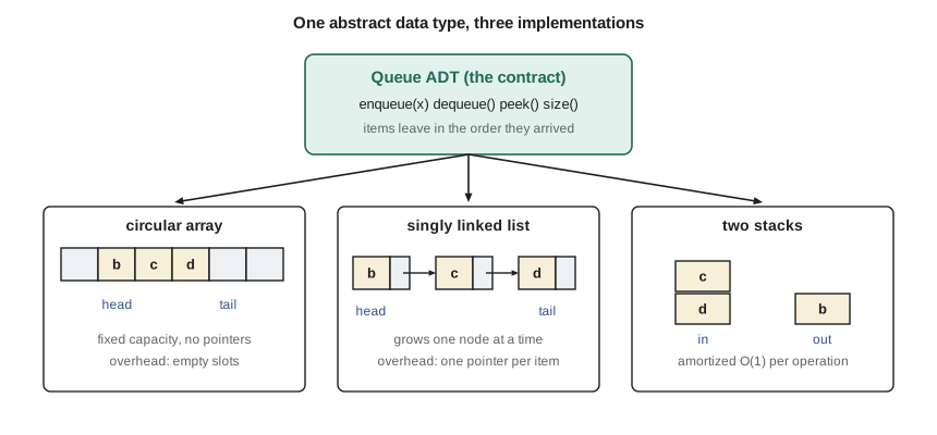
This separation matters in engineering practice for three reasons. First, it lets a team change an implementation without touching the code that uses it: when Northway moved its server from a list of records to an indexed table, none of the reporting code changed. Second, it lets you reason about correctness at the level of the contract: if the queue promises first-in, first-out order, the code that relies on that order is correct whatever happens inside. Third, it forces you to write down what each operation is supposed to do, including the awkward cases. What does dequeue do when the queue is empty? Raise an error, return a special value, or block until something arrives? On the server a Python exception is fine. On the node, an exception may reset the whole device, so the firmware returns a status code instead.
In Python, the built-in list, dict, set and collections.deque are ready-made data structures, each an implementation of one or more ADTs. In C there are none built in beyond the array, so firmware engineers write their own or use a small library, and they must understand exactly what each operation costs. This course does both. You will use Python to experiment, count operations and test ideas quickly, and you will read C listings that show how the same structures are laid out in memory on a microcontroller, where every byte and every pointer is visible.
| Abstract data type | Core operations | Typical implementations |
|---|---|---|
| List (sequence) | get by position, insert, delete, append | Dynamic array, linked list |
| Stack | push, pop, peek | Array, linked list |
| Queue | enqueue, dequeue, peek | Circular array, linked list |
| Priority queue | insert, remove the smallest (or largest) | Binary heap |
| Map (dictionary) | put key and value, get by key, delete | Hash table, balanced search tree |
| Set | add, remove, test membership | Hash table, balanced search tree, bit array |
| Graph | add vertex, add edge, list neighbours | Adjacency list, adjacency matrix |
The cost of an operation
To compare implementations you need a way to measure cost. The obvious measure is time on a stopwatch, and engineers do measure real running time, but a stopwatch result depends on the processor, the compiler, the cache, the operating system and what else is running. A more portable measure is to count basic operations: comparisons, assignments, memory reads and writes, arithmetic steps. Each takes roughly constant time on any machine. If one algorithm performs 20 comparisons to find an item and another performs 10,000, the first will win on any reasonable computer, and the counts tell you why. The cost of an operation is therefore described as a function of the input size, usually written n: the number of items in the structure, the length of the array or the number of vertices in the graph.
Costs are usually stated for three cases. The worst case is the largest number of steps the operation can take for any input of size n. It is the guarantee: a real-time system, such as the NS-4's sampling loop, must meet its deadline in the worst case, not on average. The average case is the expected number of steps over some distribution of inputs, for example searching for a key that is equally likely to be anywhere. The best case is the smallest number of steps, which is rarely useful on its own because almost any algorithm is fast on some lucky input. A fourth idea, amortized cost, describes the average cost per operation over a long sequence of operations, even when an occasional operation is expensive. Lesson 3 uses it to explain why appending to a dynamic array is cheap even though the array sometimes has to be copied.
Worked problem
Counting the cost of a search
Jonah stores the 600 vehicle records from the last ten minutes in an array in arrival order. Maren asks how many timestamp comparisons a linear search makes to find the record for a given vehicle in the best, worst and average case, assuming the vehicle is equally likely to be any of the 600 and is always present.
Show solution
- A linear search compares the target with records one at a time from the front until it finds a match.
- Best case: the target is the first record, so one comparison is made.
- Worst case: the target is the last record, so all n records are compared.
- \[C_{\text{worst}} = n = 600\]
- Average case: if the target is equally likely to be in any of the n positions, position i costs i comparisons.
- \[C_{\text{avg}} = \frac{1}{n}\sum_{i=1}^{n} i = \frac{n+1}{2} = \frac{601}{2} = 300.5\]
Answer: 1 comparison in the best case, 600 in the worst and about 300 on average. Doubling the number of records doubles both the worst and the average cost: the cost grows in proportion to n.
The example shows the key idea of the next lesson in miniature. The exact numbers, 600 and 300.5, matter less than the shape of the cost: it grows in direct proportion to the number of records. If the server held 6 million records instead of 600, a linear search would take thousands of times longer, and no faster processor would rescue it. A different structure, a hash table or a search tree, keeps the cost of finding a record almost flat as n grows. Choosing that structure is a design decision that matters far more than any micro-optimization of the search loop.
Memory is a cost too
Time is not the only cost. Each structure also uses memory, and the extra memory beyond the data itself is called overhead. An array of 600 records of 12 bytes uses 7,200 bytes and nothing more. A linked list of the same records adds a pointer to each record, 4 bytes on a 32-bit microcontroller and 8 bytes on a 64-bit server, so its overhead is a third or two thirds of the data. A hash table typically keeps 25 to 50 percent of its slots empty so that lookups stay fast. On the server these overheads hardly matter. On the NS-4, with 64 KB of RAM shared between the radar processing, the modem driver, the record buffer and the stack, they decide what is possible. Firmware engineers often avoid dynamic memory allocation altogether, because the heap can fragment over months of operation until an allocation fails. They reserve fixed-size pools at start-up and build their structures inside them.
There is also a subtler cost: the order in which memory is touched. Modern processors read memory in blocks called cache lines, typically 32 or 64 bytes, and keep recently used lines in a small, fast cache. Walking through an array touches consecutive addresses, so each cache line fetched serves several elements, and the processor can prefetch the next line before it is needed. Walking through a linked list follows pointers to wherever each node happened to be allocated, so nearly every step can be a cache miss that costs tens or hundreds of cycles on a large processor. Two structures with the same operation count can therefore differ several-fold in real speed. Lesson 3 returns to this when comparing arrays with linked lists.
# Count comparisons for a linear search over records stored in arrival order
import random

random.seed(4)
records = [(t, random.choice("CTB")) for t in range(600)]   # (timestamp, class)

def linear_search(recs, ts):
    comparisons = 0
    for i, (t, _) in enumerate(recs):
        comparisons += 1
        if t == ts:
            return i, comparisons
    return -1, comparisons

for target in (0, 299, 599):
    pos, c = linear_search(records, target)
    print(f"timestamp {target:3d}: found at index {pos:3d} after {c:3d} comparisons")

total = sum(linear_search(records, t)[1] for t in range(600))
print(f"average over all 600 targets: {total / 600:.1f} comparisons")timestamp 0: found at index 0 after 1 comparisons timestamp 299: found at index 299 after 300 comparisons timestamp 599: found at index 599 after 600 comparisons average over all 600 targets: 300.5 comparisons
The program confirms the hand count: 1, 300 and 600 comparisons for the first, middle and last records, and an average of 300.5. Counting operations in code like this is a habit worth building. It turns an abstract claim about cost into a number you can check, and when you later change the data structure you can rerun the same count and see the improvement directly. Wall-clock timing is still useful, especially for cache effects, but timings vary from run to run, so the experiments in this course count operations whenever possible and treat timings as rough confirmation.
Choosing a structure: a first look
Maren's rule for choosing a structure is to start from the operations, not from the structure. Write down every operation the program performs on the data, estimate how often each happens and how large the data gets, note any hard limits on time or memory, and only then look for the structure whose cheap operations match. For the NS-4 record buffer the list is short: append a new record up to 50 times a second, remove the oldest record after each successful upload, and never use more than a fixed 24 KB. A circular array does all three in constant time with zero overhead. For the server's lookup of a node by its serial number, the operations are put and get by key, thousands of times a minute, over 800 nodes: a hash table. For the server's daily report of the slowest 100 vehicles out of millions, the operation is keeping the largest 100 values seen so far: a heap. You will meet each of these structures in turn.
/* NS-4 vehicle record: 12 bytes, packed for the record buffer */
#include <stdint.h>

typedef struct {
    uint32_t timestamp_ms;   /* milliseconds since midnight          */
    uint16_t speed_dkmh;     /* speed in tenths of km/h               */
    uint8_t  lane;           /* 1..4                                  */
    uint8_t  vclass;         /* vehicle class code                    */
    uint32_t length_mm;      /* measured vehicle length               */
} vehicle_rec_t;

/* 24 KB reserved at start-up: 2048 records, no heap allocation */
#define REC_CAPACITY 2048
static vehicle_rec_t rec_pool[REC_CAPACITY];
Common mistakes
MistakeChoosing a data structure first and then forcing the program to fit it.
InsteadList the operations, their frequencies and the data size first; then choose the structure whose cheap operations match the common ones.
MistakeTreating an abstract data type and its implementation as the same thing.
InsteadThe ADT is the contract of operations; the data structure is one way to keep that contract. Code that uses the contract should not depend on the layout.
MistakeQuoting only the best-case cost of an operation.
InsteadState the worst case for guarantees and the average or amortized case for typical performance; the best case alone says almost nothing.
MistakeMeasuring speed with a single stopwatch run and treating it as exact.
InsteadCount operations for a portable comparison, and repeat timings several times; caches, other processes and clock frequency all change wall-clock results.
MistakeIgnoring memory overhead on an embedded target.
InsteadAdd up the data, the pointers and the empty slots. On a microcontroller, overhead and heap fragmentation can matter more than speed.
Summary and key terms
- A data structure is a way of arranging data in memory so that certain operations are cheap; an algorithm is a precise sequence of steps that works on that data.
- An abstract data type specifies the operations and their behaviour; a data structure implements it with a concrete layout.
- The cost of an operation is measured by counting basic steps as a function of the input size n, in the worst, average or amortized case.
- Memory overhead and the pattern of memory access are costs too, and they dominate on small embedded systems and in cache-sensitive code.
- Choose a structure by listing the operations the program performs, how often and on how much data, and matching them to the structure's cheap operations.
- Data structure
- A concrete arrangement of data in memory together with the operations that work on it.
- Algorithm
- A finite, precise sequence of steps that solves a problem.
- Abstract data type (ADT)
- A specification of a collection of values and the operations on it, without a commitment to any memory layout.
- Worst case
- The largest number of steps an operation can take on any input of a given size.
- Amortized cost
- The average cost per operation over a long sequence of operations, even when some individual operations are expensive.
- Overhead
- Memory a structure uses beyond the data itself, such as pointers and empty slots.
- Cache line
- The block of memory, typically 32 or 64 bytes, that a processor fetches into its cache at once.
Practice problems
Work each problem on paper first, then reveal the answer to check.
Name the ADT and a suitable structure for a printer's job list, where jobs are printed in the order they arrive.
Show answer
A queue, implemented with a circular array or a linked list.
A linear search runs over 2,000 records. How many comparisons in the worst case and on average, if the target is always present and equally likely anywhere?
Show answer
2,000 in the worst case and (2,000 + 1)/2 = 1,000.5 on average.
A linked list of 1,000 records of 12 bytes uses 4-byte pointers. What is its overhead as a percentage of the data?
Show answer
4,000 bytes on 12,000 bytes, about 33 %.
Why does the NS-4 firmware avoid dynamic memory allocation?
Show answer
Because over months of operation the heap can fragment until an allocation fails, so fixed pools reserved at start-up are safer.
Give one reason to state worst-case rather than average-case cost for a real-time sampling loop.
Show answer
The loop must meet its deadline every time, so the guarantee that matters is the worst case.
Lesson quiz · 5 questions
Score 60% or more to complete this lesson.
Create a free account to save your progress, take quizzes and earn a certificate.