
CIV-370 · Lesson 9 of 12 · 20 min
Runoff: the rational method and time of concentration
For a small, mostly paved drainage area, such as a parking lot, a building site or a short length of street, engineers usually need only one number: the peak flow that a ditch, gutter, inlet or pipe must carry. The rational method gives it in a single line. It is the oldest runoff formula in use, introduced to North American practice by Emil Kuichling in 1889 and in Britain by Lloyd-Davies in 1906, and despite its simplicity it remains the standard for sizing minor drainage systems in municipal design manuals across Canada and the United States. This lesson develops the method, the time of concentration on which it depends, and its application to the Kestrel Bay site before and after development.
The rational formula
The rational method states that the peak runoff from a small area equals a fraction of the rainfall intensity times the area:
where \(C\) is a dimensionless runoff coefficient and \(i\) is the average rainfall intensity for a duration equal to the time of concentration of the area, at the chosen return period. In US units the conversion factor is 1.008, so close to 1 that it is ignored.
The reasoning behind the formula is straightforward. Suppose rain of constant intensity falls on an area for a long time. Runoff from the nearest part reaches the outlet first, and runoff from progressively more distant parts arrives later. Once the rain has lasted as long as the time it takes water to travel from the most remote point of the area to the outlet, the whole area contributes at once, and the outflow reaches its maximum. That travel time is the time of concentration \(t_c\). A storm shorter than \(t_c\) has a higher intensity but never gets the whole area contributing; a longer storm has the whole area contributing but at a lower intensity. The peak occurs for a storm of duration equal to \(t_c\), which is why the IDF intensity is read at that duration.
The method assumes that the rainfall is uniform over the area and constant over the duration \(t_c\), that the runoff coefficient is constant, and that the return period of the peak flow equals that of the rainfall. These assumptions are reasonable for small areas and break down for larger ones. Most manuals limit the method to areas of a few tens of hectares or about a hundred acres, and some to less; larger or more complex areas need a hydrograph method, as in lesson 10. The rational method also gives only a peak, not a volume, so on its own it cannot size storage.
The runoff coefficient
The runoff coefficient lumps together all the abstractions of lesson 8 and the attenuation of the flow. It depends mainly on the surface. Typical values are listed below; design manuals give their own tables, which should be used where they apply.
| Surface | Runoff coefficient C (typical range) |
|---|---|
| Roofs | 0.75 to 0.95 |
| Asphalt and concrete pavement | 0.70 to 0.95 |
| Gravel surfaces | 0.40 to 0.70 |
| Lawns on clayey soil, flat to steep | 0.13 to 0.35 |
| Lawns on sandy soil, flat to steep | 0.05 to 0.20 |
| Woodland and forest | 0.05 to 0.25 |
| Pasture and meadow | 0.10 to 0.35 |
For an area with several surfaces, an area-weighted coefficient is used. Because the abstractions are a smaller fraction of a large storm, many manuals increase \(C\) for rare storms with a frequency factor, commonly 1.1 for the 25-year storm, 1.2 for the 50-year and 1.25 for the 100-year, with the product capped at 1.0.
Time of concentration
The time of concentration is the sum of the travel times along the longest hydraulic path, which typically has three parts: sheet flow over the surface at the top of the path, shallow concentrated flow in rills, gutters and small swales, and channel flow in ditches, pipes and streams.
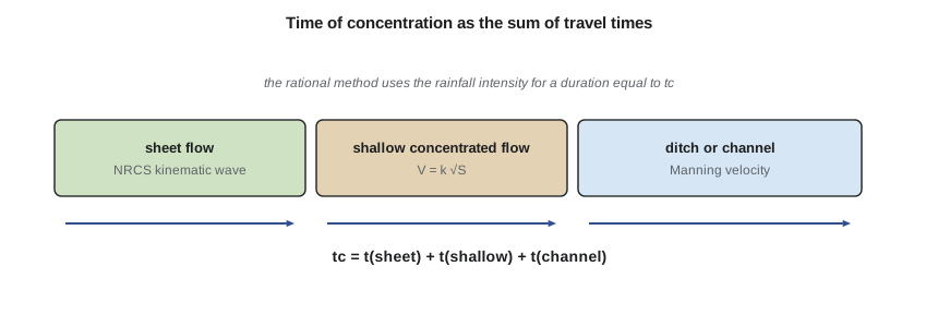
Sheet flow is the thin, often laminar flow noted in lesson 1. It is slow, and over a grassed surface it can account for most of the time of concentration even though it covers only the first few tens of metres. The NRCS method, based on kinematic wave theory, gives its travel time as
where \(n\) is a roughness coefficient for sheet flow (about 0.011 for smooth pavement and 0.24 for dense grass), \(L\) is the flow length, limited by NRCS to about 30 m or 100 ft, \(P_2\) is the 2-year, 24-hour rainfall depth and \(S\) is the slope. After that distance, flow concentrates. The NRCS gives its average velocity as \(V = 4.92\sqrt{S}\) m/s on unpaved surfaces and \(6.20\sqrt{S}\) m/s on paved ones (16.13 and 20.33 ft/s). Channel flow velocities come from Manning's equation at the bankfull or design depth, as in lesson 3.
Many empirical formulas lump the whole path into one equation. The Kirpich formula, developed in 1940 from small agricultural watersheds in Tennessee with well-defined channels, gives \(t_c = 0.0195L^{0.77}S^{-0.385}\) minutes with \(L\) in metres (or \(0.0078L^{0.77}S^{-0.385}\) with \(L\) in feet). The FAA formula, developed for airfields, the Bransby Williams formula, used in some Canadian manuals, and the kinematic wave formula are others. They give very different answers for the same area, because each was calibrated on particular conditions. Designers should use the method their approving authority prefers and check that it suits the site; the segmental method is the most transparent.
Development shortens the time of concentration dramatically. Pavement is smoother than grass, gutters and pipes replace swales, and the flow path is often straightened. A shorter \(t_c\) means a higher design intensity, so development increases peak flows both by raising \(C\) and by raising \(i\).
Kestrel Bay before and after development
Owen traces the longest flow path across the site on the topographic survey. Before development, it begins with 30 m of sheet flow over dense grass at 2 %, continues 170 m as shallow concentrated flow at 1.5 % and ends with 250 m in a shallow natural swale flowing at about 0.5 m/s. After development, the path begins with 30 m of sheet flow over pavement at 1 %, then 120 m of gutter flow at 1 %, and ends with 300 m in the new perimeter ditch at about 1.1 m/s, the velocity computed in lesson 3. The 2-year, 24-hour rainfall used in the sheet flow formula is taken as 30 mm for this illustration.
Worked problem
The 100-year peak after development
After development, the site of 7.5 ha has a weighted runoff coefficient of 0.68 and a time of concentration of 10 minutes. Find the 100-year peak flow using the course IDF relation \(i = 1340/(t + 6)^{0.8}\) mm/h and a frequency factor of 1.25.
Show solution
- Intensity at the time of concentration:
- \[i = \frac{1340}{(10.3 + 6)^{0.8}} = 143\ \text{mm/h}\]
- Peak flow, with \(C_f C = 1.25 \times 0.68 = 0.85\):
- \[Q = 0.00278(0.85)(143)(7.5) = 2.55\ \text{m}^3/\text{s}\]
Answer: The developed site would deliver about 2.55 m³/s at the 100-year peak if nothing were done. The perimeter ditch is sized for the 25-year peak of 1.85 m³/s; larger storms are carried by the yard grading as an overland route to the pond, which Anika checks separately.
Sofia's script computes the segment travel times before and after development, compares a Kirpich estimate, finds the weighted runoff coefficient from the planned surfaces and tabulates peak flows for five return periods.
# Rational method for the Kestrel Bay site, with time of concentration by segments
from math import sqrt
UNITS = "SI"
SI = UNITS == "SI"
a, b, c = 1340.0, 6.0, 0.80                      # 100-year IDF from lesson 7, i in mm/h, t in min
scale = {2: 0.42, 5: 0.58, 10: 0.69, 25: 0.82, 50: 0.91, 100: 1.00}
def i_mm(t, T): return scale[T] * a / (t + b) ** c
# NRCS segmental travel time; lengths in m (SI) or ft (US)
P2 = 30.0 if SI else 30.0 / 25.4                 # 2-year 24-hour rain, illustrative
def sheet(n, Lf, s):                             # NRCS sheet flow, minutes
    if SI:  return 60 * 0.091 * (n * Lf) ** 0.8 / ((P2) ** 0.5 * s ** 0.4)      # P2 in mm, L in m
    return 60 * 0.007 * (n * Lf) ** 0.8 / (P2 ** 0.5 * s ** 0.4)                # P2 in in., L in ft
def shallow(Lf, s, paved):                       # shallow concentrated flow velocity
    V = (6.20 if paved else 4.92) * sqrt(s) if SI else (20.33 if paved else 16.13) * sqrt(s)
    return Lf / V / 60
def channel(Lf, V): return Lf / V / 60
if SI:
    A, ua, uq, k = 7.5, "ha", "m3/s", 0.00278    # Q = 0.00278 C i A, i in mm/h, A in ha
    pre = [sheet(0.24, 30, 0.02), shallow(170, 0.015, False), channel(250, 0.5)]
    post = [sheet(0.011, 30, 0.01), shallow(120, 0.01, True), channel(300, 1.1)]
else:
    A, ua, uq, k = 18.5, "acres", "cfs", 1.0     # Q = C i A, i in in./h, A in acres
    pre = [sheet(0.24, 100, 0.02), shallow(560, 0.015, False), channel(820, 1.6)]
    post = [sheet(0.011, 100, 0.01), shallow(390, 0.01, True), channel(980, 3.6)]
tc_pre, tc_post = sum(pre), sum(post)
print("Travel times (min): pre", [round(t, 1) for t in pre], "post", [round(t, 1) for t in post])
print(f"tc before development = {tc_pre:.0f} min, after = {tc_post:.0f} min")
# Kirpich for comparison (pre-development, total length and fall)
Lk = 450 if SI else 1480; H = 6.0 if SI else 20.0
tk = 0.0195 * Lk ** 0.77 * (Lk / H) ** 0.385 if SI else 0.0078 * Lk ** 0.77 * (Lk / H) ** 0.385
print(f"Kirpich estimate before development: {tk:.0f} min")
cover = [("Roofs", 0.18, 0.95), ("Pavement and yard", 0.42, 0.90), ("Gravel storage", 0.10, 0.60), ("Lawn and landscaping", 0.30, 0.25)]
C_post = sum(f * cc for _, f, cc in cover); C_pre = 0.25
print(f"Runoff coefficient: before {C_pre:.2f}, after {C_post:.2f}")
print(f"{'T':>4} {'Cf':>5} {'i_pre':>7} {'Q_pre':>7} {'i_post':>7} {'Q_post':>7}")
for T in (2, 5, 10, 25, 100):
    Cf = {25: 1.1, 50: 1.2, 100: 1.25}.get(T, 1.0)     # frequency factor for rare storms
    ip, iq = i_mm(tc_pre, T), i_mm(tc_post, T)
    if not SI: ip, iq = ip / 25.4, iq / 25.4
    Qp = k * min(1.0, C_pre * Cf) * ip * A; Qq = k * min(1.0, C_post * Cf) * iq * A
print(f"{T:4d} {Cf:5.2f} {ip:7.2f} {Qp:7.2f} {iq:7.2f} {Qq:7.2f}")Travel times (min): pre [23.1, 4.7, 8.3] post [2.6, 3.2, 4.5] tc before development = 36 min, after = 10 min Kirpich estimate before development: 11 min Runoff coefficient: before 0.25, after 0.68 T Cf i_pre Q_pre i_post Q_post 2 1.00 28.21 0.15 60.16 0.86 5 1.00 38.96 0.20 83.07 1.18 10 1.00 46.35 0.24 98.83 1.41 25 1.10 55.08 0.32 117.45 1.84 100 1.25 67.17 0.44 143.23 2.55
Reading the results
The time of concentration falls from 36 minutes before development to 10 minutes after. Before development, sheet flow over grass takes 23 of the 36 minutes; after development, sheet flow over pavement takes under 3. The weighted runoff coefficient rises from 0.25 to 0.68. Together, these changes multiply the peak flow by about six for every return period: the 100-year peak rises from 0.44 m³/s to 2.55 m³/s. The Kirpich formula would estimate only 11 minutes for the undeveloped site, because it was calibrated on channelized watersheds where sheet flow is a small part of the path; using it here would overstate the pre-development peak and, with it, the release rate the city would allow from the pond.
The pre-development peaks set the allowable release from the pond: 0.15 m³/s for the 2-year storm up to 0.44 m³/s for the 100-year storm. Lesson 10 routes a full post-development hydrograph through the pond and its outlet to show that the release stays below these values.
Minor and major systems
Urban drainage in North America is designed as two systems. The minor system, consisting of gutters, inlets, storm sewers and small ditches, carries frequent storms, typically up to the 2- to 10-year event in streets and somewhat more on private sites, so that traffic and daily use are not disrupted. The major system, consisting of the streets themselves, overland flow routes, swales and ponds, carries the rare storms, up to the 100-year event, without flooding buildings. Both must be designed: a perfectly sized storm sewer is no help if the overland route for a larger storm leads into a basement. At Kestrel Bay, the perimeter ditch is the minor system, and the graded yard sloping toward the pond is the major system. The building floors are set at least 0.3 m (1 ft) above the 100-year overland flow level.
Using the rational method for pipes
For a storm sewer network, the rational method is applied progressively from the top of the system down. At each inlet, the time of concentration is the longest of the inlet time and the times along each upstream path, including travel time in the pipes. The peak flow is computed with the accumulated sum of \(CA\) for all tributary areas and the intensity for that time. The pipe is then sized by Manning's equation for full flow, and the velocity in it is used to add travel time for the next reach. CIV-440 develops storm sewer design in detail.
Practical points
- Use the rational method for small areas only, within the limit set by the approving authority.
- Compute the time of concentration segment by segment; sheet flow often dominates on grassed areas.
- Use a frequency factor on \(C\) for rare storms, capped at 1.0.
- Check that the whole area produces the largest peak; sometimes a smaller, more impervious part with a short \(t_c\) gives a higher peak alone.
- Remember that the method gives a peak, not a volume; use a hydrograph method to size storage.
Common mistakes
MistakeUsing the same time of concentration before and after development.
InsteadDevelopment shortens \(t_c\) and so raises the design intensity.
MistakeApplying an empirical \(t_c\) formula outside the conditions it was derived for.
InsteadUse the segmental method, or a formula suited to the site.
MistakeUsing the rational method to size a detention pond.
InsteadIt gives only a peak; storage needs a hydrograph.
MistakeAllowing sheet flow over long distances.
InsteadLimit sheet flow to about 30 m or 100 ft; beyond that it concentrates.
Summary and key terms
- Rational method: \(Q = 0.00278CiA\) (SI) or \(Q = CiA\) (US), with \(i\) at duration \(t_c\).
- \(C\) depends on the surface; increase it for rare storms with a frequency factor.
- \(t_c\) is the sum of sheet, shallow concentrated and channel flow travel times.
- Development raises \(C\) and shortens \(t_c\), multiplying peak flows.
- Kestrel Bay: \(t_c\) 36 → 10 min, \(C\) 0.25 → 0.68, 100-year peak 0.44 → 2.55 m³/s.
- Drainage has a minor system for frequent storms and a major system for rare ones.
- Rational method
- A formula giving the peak runoff from a small area as the product of a runoff coefficient, intensity and area.
- Runoff coefficient
- The ratio of peak runoff rate to rainfall rate in the rational method.
- Time of concentration
- The time for runoff to travel from the hydraulically most remote point of a drainage area to its outlet.
- Sheet flow
- Shallow flow over a plane surface at the top of a flow path.
- Shallow concentrated flow
- Flow in rills, gutters and small swales after sheet flow concentrates.
- Minor system
- The gutters, inlets, sewers and ditches that carry frequent storms.
- Major system
- The streets, overland routes and ponds that carry rare storms safely.
Practice problems
Work each problem on paper first, then reveal the answer to check.
A 2.0 ha parking lot (C = 0.90) has a time of concentration of 8 min. Find the 10-year peak with the course IDF relation (10-year ratio 0.69).
Show answer
\(i = 0.69 \times 1340/14^{0.8} = 112\) mm/h; \(Q = 0.00278(0.90)(112)(2.0) = 0.56\) m³/s.
A site has 40 % roof (C 0.90), 30 % pavement (C 0.85) and 30 % lawn (C 0.20). Find the weighted C.
Show answer
\(0.40(0.90) + 0.30(0.85) + 0.30(0.20) = 0.675\).
Find the travel time of shallow concentrated flow over 200 m of unpaved ground at 2 %.
Show answer
\(V = 4.92\sqrt{0.02} = 0.70\) m/s; \(t = 200/0.70 = 290\) s, about 4.8 min.
Why does the peak from a drainage area occur for a storm whose duration equals the time of concentration?
Show answer
Shorter storms are more intense but never get the whole area contributing; longer storms get the whole area contributing but at a lower intensity.
Lesson quiz · 5 questions
Score 60% or more to complete this lesson.
Create a free account to save your progress, take quizzes and earn a certificate.