Flood frequency analysis and climate change

Lesson 10 estimated the 100-year flood of Kestrel Creek by building it from a design storm. That approach assumes that a 100-year storm produces a 100-year flood, which is only roughly true: the flood also depends on how wet the watershed is, on snowmelt and on the storm's pattern. Where streamflow has been measured for many years, the flood can instead be estimated directly from the record by statistical analysis. This lesson applies flood frequency analysis to a regional gauge, transfers the result to the ungauged creek, compares it with the hydrograph estimate, and then asks how a changing climate affects a design that must serve for decades.

Streamflow records

In Canada, the Water Survey of Canada, part of Environment and Climate Change Canada, operates the national network of hydrometric stations in partnership with the provinces, and publishes its data in the HYDAT database. Each station measures water level continuously and converts it to discharge through a rating curve, built from periodic measurements of flow, as described in lesson 6. Many small streams, including Kestrel Creek, have no gauge, but a gauged creek of similar character nearby can serve as a model.

For flood analysis, the largest instantaneous peak flow in each water year forms the annual maximum series, just as for rainfall in lesson 7. A partial duration series, which includes every peak above a threshold, is sometimes used for frequent floods. The record must be checked for homogeneity: changes in the watershed, such as urbanization, dams or drainage works, and changes in the gauge or its rating can make early and late years incomparable.

Plotting positions

Before fitting a distribution, the recorded peaks are ranked from largest to smallest and plotted against an empirical estimate of their return period. The Weibull plotting position assigns the \(m\)th largest of \(n\) values a return period

Other formulas, such as Cunnane's, \(T = (n + 0.2)/(m - 0.4)\), are less biased for particular distributions. Plotting the data on probability paper, where a chosen distribution appears as a straight line, shows at a glance how well the distribution fits and whether any points are outliers.

Distributions and the frequency factor

Many distributions have been used for floods. Chow showed in 1951 that most can be written in the same frequency factor form as the Gumbel distribution of lesson 7:

where \(K_T\) depends on the distribution, the return period and, for three-parameter distributions, the skew. The Gumbel distribution has a fixed skew of 1.14. The log-Pearson type III (LP3) distribution applies the Pearson type III distribution to the logarithms of the flows, with three parameters: the mean, standard deviation and skew coefficient of the logs. Its frequency factor is tabulated against skew and return period, or approximated by the Wilson-Hilferty transformation:

where \(G\) is the skew coefficient and \(z\) the standard normal variate for the non-exceedance probability \(1 - 1/T\). When \(G = 0\), the LP3 distribution becomes the log-normal distribution and \(K_T = z\).

Canada has no single national standard method. Practice, reflected in provincial technical guides and in federal flood mapping guidance, is to fit several candidate distributions, commonly the generalized extreme value, three-parameter log-normal, Pearson type III and log-Pearson type III, check their fit graphically and statistically, and select one with judgement, often favouring regional consistency. Ontario's technical guidance on river and stream flooding hazards describes acceptable approaches.

Uncertainty

A 40-year record gives a reasonable estimate of the 10-year flood and a much less certain estimate of the 100-year flood, which lies beyond the range of the data. Confidence intervals widen rapidly with return period. The skew coefficient in particular is poorly determined from short records, which is why regional skews are used. A single extreme flood in a short record can change the estimate substantially, as can the choice of distribution. Engineers should report the uncertainty and, for important structures, check a range of estimates rather than a single number.

Transferring to an ungauged site

Flows estimated at a gauge are transferred to an ungauged site on a similar stream by an area ratio:

where the exponent \(b\) is commonly between 0.5 and 1, and about 0.7 to 0.8 for flood peaks in many regions; smaller watersheds produce more flow per unit area because storms cover them completely and their response is quicker. Regional regression equations, which relate flood quantiles to drainage area, slope, storage and climate across many gauges, are a more refined method. The transfer is reliable only when the two watersheds are similar in climate, soils, slope and storage, and the area ratio is not extreme.

The regional gauge

About 20 km from the site, a gauged creek with a watershed of 48 km² drains similar forest and pasture over the same glacial lake deposits. Anika obtains its 40-year record of annual peaks. For this course the record is illustrative, generated for teaching rather than taken from an actual station.

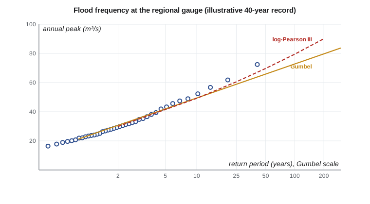
Sofia's script computes the statistics, the plotting positions of the largest floods, the Gumbel and LP3 quantiles, the transfer to Kestrel Creek and the effect of an increase in storm rainfall on runoff.

# Flood frequency analysis of a regional gauge and transfer to Kestrel Creek
from math import log10, sqrt, log, pi, exp
UNITS = "SI"
SI = UNITS == "SI"
cf = 1.0 if SI else 35.315; uq = "m3/s" if SI else "cfs"
# Illustrative 40-year annual peak series at a gauge on a nearby creek, 48 km2 (m3/s)
peaks = [31.2, 22.8, 45.6, 18.9, 27.4, 38.1, 24.5, 52.3, 20.1, 29.8, 34.7, 16.4, 41.9, 26.3, 23.7, 61.8,
         28.5, 19.6, 33.2, 47.4, 25.1, 21.9, 36.6, 30.4, 17.8, 43.3, 27.9, 24.0, 56.7, 32.5, 22.1, 39.4,
         26.8, 20.7, 35.3, 29.1, 48.9, 23.3, 31.7, 72.4]
x = [p * cf for p in peaks]; n = len(x)
mean = sum(x) / n; sd = sqrt(sum((v - mean) ** 2 for v in x) / (n - 1))
def KG(T): return -sqrt(6) / pi * (0.5772 + log(log(T / (T - 1))))
def z(p):                                      # standard normal quantile (Abramowitz and Stegun 26.2.23)
    q = p if p < 0.5 else 1 - p
    t = sqrt(-2 * log(q))
    zz = t - (2.515517 + 0.802853 * t + 0.010328 * t * t) / (1 + 1.432788 * t + 0.189269 * t * t + 0.001308 * t ** 3)
    return -zz if p < 0.5 else zz
y = [log10(v) for v in x]
my = sum(y) / n; sy = sqrt(sum((v - my) ** 2 for v in y) / (n - 1))
G = n * sum((v - my) ** 3 for v in y) / ((n - 1) * (n - 2) * sy ** 3)
def KP(T, g):                                  # Wilson-Hilferty frequency factor for Pearson type III
    zz = z(1 - 1 / T); k = g / 6
    return zz if abs(g) < 1e-6 else (2 / g) * ((1 + k * zz - k * k) ** 3 - 1)
print(f"Gauge: n = {n}, mean {mean:.{1 if SI else 0}f} {uq}, sd {sd:.{1 if SI else 0}f}; logs: mean {my:.4f}, sd {sy:.4f}, skew {G:.3f}")
srt = sorted(x, reverse=True)
print("Largest three, Weibull return periods:", ", ".join(f"{v:.{1 if SI else 0}f} ({(n + 1) / (m + 1):.0f} yr)" for m, v in enumerate(srt[:3])))
print(f"{'T':>4} {'Gumbel':>8} {'LP3':>8}")
for T in (2, 10, 25, 50, 100, 200):
    print(f"{T:4d} {mean + KG(T) * sd:8.{1 if SI else 0}f} {10 ** (my + KP(T, G) * sy):8.{1 if SI else 0}f}")
Q100 = 10 ** (my + KP(100, G) * sy)
Ag, As = (48.0, 6.4) if SI else (18.5, 2.5)     # drainage areas, km2 or mi2 (gauge, Kestrel Creek)
r = (As / Ag) ** 0.75
print(f"\nTransfer to Kestrel Creek by (A/Ag)^0.75 = {r:.3f}: Q100 = {Q100 * r:.{1 if SI else 0}f} {uq}")
print(f"Unit hydrograph estimate (lesson 10): {17.8 if SI else 638} {uq}")
# climate change: rainfall +15 % and its effect on runoff depth with CN 75
def runoff(P, CN):
    S = 25400 / CN - 254; Ia = 0.2 * S
    return 0.0 if P <= Ia else (P - Ia) ** 2 / (P - Ia + S)
P = 71.5
for inc in (0.0, 0.10, 0.15, 0.20):
    q = runoff(P * (1 + inc), 75)
    print(f"rain +{inc * 100:3.0f} %: runoff {q / (1 if SI else 25.4):.{1 if SI else 2}f} {'mm' if SI else 'in.'}, change {q / runoff(P, 75) * 100 - 100:+.0f} %")

Gauge: n = 40, mean 32.8 m3/s, sd 12.8; logs: mean 1.4869, sd 0.1553, skew 0.462
Largest three, Weibull return periods: 72.4 (41 yr), 61.8 (20 yr), 56.7 (14 yr)
   T   Gumbel      LP3
   2     30.7     29.9
  10     49.4     49.2
  25     58.8     60.5
  50     65.8     69.7
 100     72.8     79.5
 200     79.7     90.1

Transfer to Kestrel Creek by (A/Ag)^0.75 = 0.221: Q100 = 17.5 m3/s
Unit hydrograph estimate (lesson 10): 17.8 m3/s
rain +  0 %: runoff 21.4 mm, change +0 %
rain + 10 %: runoff 26.0 mm, change +22 %
rain + 15 %: runoff 28.4 mm, change +33 %
rain + 20 %: runoff 30.9 mm, change +44 %

Reading the results

The two distributions agree closely up to about the 10-year flood, near 49 m³/s, and diverge above it: at 100 years, Gumbel gives 72.8 m³/s and LP3 gives 79.5 m³/s. The largest recorded flood, 72.4 m³/s, has a Weibull return period of 41 years; the LP3 curve passes closer to the largest floods, which is one reason to prefer it here. Transferring the LP3 value to Kestrel Creek with an exponent of 0.75 gives 17.5 m³/s, remarkably close to the 17.8 m³/s from the unit hydrograph. Two independent methods agree within 2 %, and Anika adopts 18 m³/s as the 100-year design flow. Such close agreement is partly luck; differences of 20 to 30 % between methods are common, and the engineer must then judge which is more reliable.

Nonstationarity and climate change

Every method in this course so far assumes stationarity: that the statistics of rainfall and floods in the future will be the same as in the past record. That assumption is now in doubt. A warmer atmosphere holds more water vapour, about 7 % more per degree Celsius according to the Clausius-Clapeyron relation, and observations and climate models indicate that the heaviest short-duration rainfalls are intensifying in many regions, including the Great Lakes basin. Snowmelt floods may decline in some places as winters warm, while rain-on-snow events and winter rain on frozen ground may increase. Land-use change, especially urbanization, adds its own trend.

Canadian practice is moving to account for this. The CSA technical guide on IDF information describes methods to adjust IDF curves for climate change, projected IDF values are available through the national climate data portal, federal flood mapping guidance asks for climate change to be considered, and some municipalities and provinces now require designers to check infrastructure with climate-adjusted rainfall or apply an uplift to design intensities. Engineers Canada's guidance and the Public Infrastructure Engineering Vulnerability Committee (PIEVC) protocol support vulnerability assessments of infrastructure to climate.

A practical approach for a project like Kestrel Bay is a sensitivity check: increase the design rainfall by a plausible amount, recompute the runoff and the flood, and see whether the design still performs or fails gracefully. The script shows why this matters: because runoff is a nonlinear function of rainfall, a 15 % increase in storm rainfall increases the runoff depth by 33 %, and the peak flow by a similar proportion. Anika therefore adds a climate check to the culvert design: a flow of 24 m³/s, about one-third above the 100-year flow. Lesson 12 tests both culverts against it.

Practical points

• Check the record for homogeneity and outliers before fitting.
• Follow the jurisdiction's method: Bulletin 17C in US federal work, or the provincial guidance in Canada.
• Compare a statistical estimate with a rainfall-runoff estimate; investigate large differences.
• Transfer flows only between similar watersheds, with a justified exponent.
• Report uncertainty and test sensitivity to climate change for long-lived infrastructure.