
CHE-345 · Lesson 2 of 12 · 21 min
Conversion and reactor sizing
The ethyl acetate line will make about 25,000 tonnes of ester a year. Ingrid's process concept puts a fixed bed of acid ion-exchange resin ahead of a reactive distillation column. The bed, called the pre-reactor, brings the mixture of acetic acid and ethanol most of the way to chemical equilibrium before the column, where removing water as the reaction proceeds pushes it past the equilibrium limit. Theo's job this week is to size the pre-reactor for a first estimate, and to say whether a tube, a stirred tank or some combination is the better choice. He uses a tool that shows the answer at a glance: the Levenspiel plot.
Design equations in terms of conversion
For a single reaction, conversion \(X\) is the natural variable. With \(F_A = F_{A0}(1 - X)\), the design equations of lesson 1 become
| Reactor | Differential form | Integral or algebraic form |
|---|---|---|
| Batch | \(N_{A0}\,dX/dt = -r_AV\) | \(t = N_{A0}\int_0^X dX/(-r_AV)\) |
| CSTR | — | \(V = F_{A0}X/(-r_A)_{\text{exit}}\) |
| PFR | \(F_{A0}\,dX/dV = -r_A\) | \(V = F_{A0}\int_0^X dX/(-r_A)\) |
| PBR | \(F_{A0}\,dX/dW = -r_A'\) | \(W = F_{A0}\int_0^X dX/(-r_A')\) |
The only missing piece is \(-r_A\) as a function of \(X\). Lessons 3 and 5 show how to build it from a rate law and stoichiometry, or how to measure it. If \(-r_A(X)\) is known, from a model or from laboratory data, the reactor can be sized without knowing anything else about the chemistry. That is what makes the next idea so useful.
The Levenspiel plot
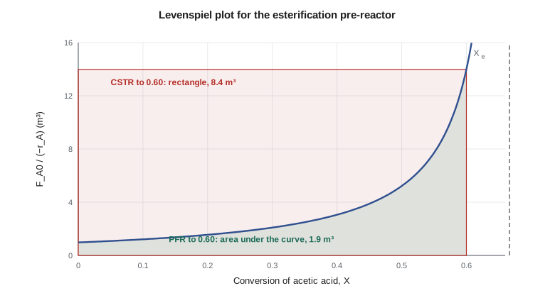
Plot \(F_{A0}/(-r_A)\) against \(X\). The PFR design equation says the PFR volume to reach conversion \(X\) is the area under that curve from 0 to \(X\). The CSTR equation says the CSTR volume is the area of a rectangle whose height is the curve's value at the exit conversion and whose width is \(X\). For any reaction whose rate falls as conversion rises, the curve rises with \(X\), and the rectangle always encloses more area than the region under the curve. The plot makes the CSTR's disadvantage visible, and it makes combinations of reactors easy to evaluate: each reactor's volume is its own slice of the diagram.
The plot is named for Octave Levenspiel, whose textbook made graphical reactor design a standard part of chemical engineering teaching from the 1960s on. Simulators now do the integration, but the plot remains the quickest way to see why a design works and where most of the volume goes.
The pre-reactor's rate
The esterification is reversible:
Lesson 11 of CHE-320 found its equilibrium constant to be about 4, so an equimolar feed can reach only two-thirds conversion. Lesson 3 derives the rate as a function of conversion; for now, take the pseudo-homogeneous form that the resin vendor's data support, written per cubic metre of packed bed:
with \(k = 1.5\times10^{-4}\) m³/(kmol s) at 80 °C, an illustrative value for a bed of acid resin, and \(C_{A0} = 8.7\) kmol/m³ for an equimolar liquid mixture. The term in brackets falls to zero at equilibrium, \(X_e = 2/3\), so \(F_{A0}/(-r_A)\) rises without limit as \(X\) approaches \(X_e\). The design feed is 40 kmol/h of acetic acid with an equal amount of ethanol.
# Levenspiel plot and reactor sizing for the esterification pre-reactor
# CH3COOH (A) + C2H5OH (B) <=> CH3COOC2H5 (C) + H2O (D), equimolar liquid feed at 80 C
# rate per unit reactor volume of resin bed (pseudo-homogeneous, illustrative constants)
K = 4.0          # equilibrium constant (about 4)
k = 1.5e-4       # m3/(kmol s) at 80 C, illustrative for a packed bed of acid resin
CA0 = 8.7        # kmol/m3 acetic acid (and ethanol) in the 1:1 mixture
FA0 = 40.0 / 3600  # kmol/s (40 kmol/h of acetic acid)

def rate(X):  # -rA, kmol/(m3 s)
    return k * CA0 ** 2 * ((1 - X) ** 2 - X ** 2 / K)

Xe = 2 / 3
print(f"equilibrium conversion Xe = {Xe:.3f}")
print("X     -rA (kmol/m3 h)   FA0/-rA (m3)")
for X in (0.0, 0.1, 0.2, 0.3, 0.4, 0.5, 0.55, 0.60):
    print(f"{X:4.2f}   {rate(X) * 3600:9.2f}         {FA0 / rate(X):7.3f}")

def simpson(f, a, b, n=200):
    h = (b - a) / n
    s = f(a) + f(b) + sum((4 if i % 2 else 2) * f(a + i * h) for i in range(1, n))
    return s * h / 3

Xt = 0.60
g = lambda X: FA0 / rate(X)
V_pfr = simpson(g, 0, Xt)
V_cstr = g(Xt) * Xt
print(f"target X = {Xt}: PFR volume {V_pfr:.2f} m3, single CSTR {V_cstr:.2f} m3")
# two equal-volume CSTRs in series reaching 0.60: find X1 by bisection so that V1 = V2
lo, hi = 0.01, Xt - 0.01
for _ in range(60):
    X1 = (lo + hi) / 2
    V1 = g(X1) * X1; V2 = g(Xt) * (Xt - X1)
    lo, hi = (X1, hi) if V1 < V2 else (lo, X1)
print(f"two equal CSTRs: X1 = {X1:.3f}, each {V1:.2f} m3, total {2 * V1:.2f} m3")
# a CSTR to X = 0.30 followed by a PFR to 0.60
Va = g(0.30) * 0.30; Vb = simpson(g, 0.30, Xt)
print(f"CSTR to 0.30 then PFR to 0.60: {Va:.2f} + {Vb:.2f} = {Va + Vb:.2f} m3")
print(f"pushing the PFR to X = 0.65 needs {simpson(g, 0, 0.65):.2f} m3")equilibrium conversion Xe = 0.667 X -rA (kmol/m3 h) FA0/-rA (m3) 0.00 40.87 0.979 0.10 33.00 1.212 0.20 25.75 1.553 0.30 19.11 2.093 0.40 13.08 3.058 0.50 7.66 5.219 0.55 5.19 7.714 0.60 2.86 13.981 target X = 0.6: PFR volume 1.90 m3, single CSTR 8.39 m3 two equal CSTRs: X1 = 0.462, each 1.92 m3, total 3.84 m3 CSTR to 0.30 then PFR to 0.60: 0.63 + 1.48 = 2.11 m3 pushing the PFR to X = 0.65 needs 3.23 m3
Reading the results
At the inlet the rate is about 41 kmol/(m³ h); at 60 % conversion it has fallen to under 3, a factor of fourteen. A PFR reaching 0.60 needs 1.9 m³ of bed. A single CSTR needs 8.4 m³, more than four times as much, because the whole tank runs at the slow rate near equilibrium. Two equal CSTRs in series need 3.8 m³ in total: the first tank works at a conversion of 0.46 where the rate is still reasonable, and only the second runs at the slow outlet rate. A CSTR to 0.30 followed by a PFR to 0.60 needs 2.1 m³, close to the pure PFR.
The last line of the output carries a design lesson of its own. Pushing the PFR from 0.60 to 0.65, a small gain in conversion, takes the bed from 1.9 to 3.2 m³. Near equilibrium, each extra percent costs more volume than the last, and at \(X_e\) the volume becomes infinite. Ingrid's concept deliberately stops the pre-reactor at about 90 % of the equilibrium conversion and lets the reactive distillation column do the rest by removing water, which moves the equilibrium itself. This is a general rule for reversible reactions: approach equilibrium sensibly, then change the conditions rather than buying volume.
Worked problem
Two reactors in series
Show, from the Levenspiel table, why two equal CSTRs to 0.60 need less volume than one.
Show solution
- One CSTR: height \(F_{A0}/(-r_A)\) at 0.60 is 13.98 m³; volume \(= 13.98 \times 0.60 = 8.39\) m³.
- Two tanks: the first reaches \(X_1 = 0.462\), where \(F_{A0}/(-r_A)\) is about 4.2 m³; volume \(= 4.2 \times 0.462 = 1.92\) m³.
- The second covers 0.462 to 0.60 at height 13.98: volume \(= 13.98 \times 0.138 = 1.92\) m³.
- Total 3.84 m³: the first tank avoids running at the slow outlet rate.
Answer: Two equal tanks need 3.8 m³, less than half of the single tank's 8.4 m³.
Reactors in series and the approach to plug flow
The two-tank result generalises. As the number of equal tanks in series grows, the staircase of rectangles fits the curve more and more closely, and the total volume approaches the PFR volume. Ten tanks are already within a few percent. This is why industrial liquid-phase processes that need good mixing, such as some polymerisations and fermentations, use cascades of stirred tanks: they keep the mixing and heat-transfer advantages of a tank while approaching the volume efficiency of a tube. Lesson 11 turns the idea around and uses a number of equivalent tanks in series to describe how far a real packed bed departs from plug flow.
Which order of reactors is best depends on the shape of the curve. For the usual monotonically rising curve, the PFR should come first in any combination of a PFR and a CSTR, and the smallest total volume is obtained with the PFR alone. For an autocatalytic reaction, or an exothermic adiabatic reactor whose rate first rises with temperature and then falls as reactant runs out, the curve has a minimum. Then a CSTR operating at the minimum followed by a PFR can beat a PFR alone. The Levenspiel plot shows which case applies at a glance.
Space time, space velocity and residence time
Two more measures appear on vendor data sheets. Space time \(\tau = V/v_0\) is the volume divided by the inlet volumetric flow. Space velocity is its reciprocal: liquid hourly space velocity (LHSV) uses the liquid feed rate at standard conditions, and gas hourly space velocity (GHSV) uses the gas feed at standard temperature and pressure. For the pre-reactor, the feed of 40 kmol/h of acid in an equimolar mixture is about 4.6 m³/h, so a 1.9 m³ bed has \(\tau\) of about 25 minutes and an LHSV of about 2.4 per hour. Resin vendors usually quote a recommended LHSV range, which gives a quick check on a design.
Residence time, the time a fluid element actually spends in the reactor, equals the space time only for a constant-density fluid in plug flow. In a CSTR the residence time is distributed, with a mean equal to \(\tau\); in a gas-phase reactor whose volume flow grows as moles are produced, the mean residence time is shorter than \(\tau\). Lesson 3 shows why.
Sizing from laboratory data
The Levenspiel method does not need a rate law at all. If the laboratory measures \(-r_A\) at a set of conversions, by running a small CSTR at several flow rates for example, the measured values of \(F_{A0}/(-r_A)\) can be plotted against \(X\) and the areas read directly. This is the safest way to size a reactor when the kinetics are complex, as they often are with catalysts and with biological reactions. The catch is that the data must be measured at the same temperature, pressure and feed composition as the design, because \(-r_A(X)\) depends on all three.
For the pre-reactor, Theo has only the vendor's rate law at 80 °C and a promise from Dev Raman in the QC lab to measure rates on the plant's own acid and ethanol. He reports the 1.9 m³ figure as a first estimate, notes that the rate constant is the vendor's and not yet confirmed, and adds the design margins Ingrid expects for catalyst ageing and non-ideal flow. Lesson 12 completes the sizing with an energy balance and those margins.
Recycle and overall conversion
The pre-reactor's per-pass conversion is not the plant's overall conversion. The reactive distillation column behind it converts most of what is left, and any acid or ethanol that leaves unreacted is separated and recycled to the front of the process. Overall conversion, based on fresh feed, can therefore approach 100 % while the single-pass conversion of any one reactor stays well below equilibrium. Recycle changes what the reactor must do: its feed now contains some product and water carried back with the recycle, which lowers the rate and the equilibrium conversion of the combined feed, as the stoichiometry of lesson 3 shows. A first estimate sizes the reactor on fresh feed alone; the design basis must then be repeated with the recycle compositions from the flowsheet.
Common mistakes
MistakeComparing reactor volumes at different conversions.
InsteadCompare reactor types at the same target conversion and the same feed.
MistakeDesigning a reversible reaction to its equilibrium conversion.
InsteadThe volume becomes infinite at \(X_e\); design to a fraction of it and change conditions to go further.
MistakeUsing a Levenspiel curve measured at another temperature.
InsteadThe curve applies only at the temperature, pressure and feed it was measured at.
MistakePutting the CSTR first when the curve rises monotonically.
InsteadFor a rising curve, put the PFR first, or use the PFR alone.
Summary and key terms
- The design equations in terms of conversion need only \(-r_A(X)\).
- On a plot of \(F_{A0}/(-r_A)\) against \(X\), the PFR volume is the area under the curve and the CSTR volume is a rectangle.
- For the pre-reactor to 60 % conversion: PFR 1.9 m³, one CSTR 8.4 m³, two CSTRs 3.8 m³.
- Near equilibrium the volume rises steeply; stop short of \(X_e\) and change conditions to go further.
- Tanks in series approach plug flow as their number grows.
- Space time is \(V/v_0\); space velocity is its reciprocal.
- Levenspiel plot
- A plot of F_A0/(−r_A) against conversion used to size reactors graphically.
- Equilibrium conversion
- The highest conversion a reversible reaction can reach at given conditions.
- Reactors in series
- Reactors arranged so that the outlet of one feeds the next.
- Space velocity
- The reciprocal of space time; LHSV and GHSV are common forms.
- Residence time
- The time a fluid element spends in a reactor.
- Pseudo-homogeneous rate
- A catalytic rate expressed per unit volume of bed as if the reaction were homogeneous.
Practice problems
Work each problem on paper first, then reveal the answer to check.
A reaction has \(F_{A0}/(-r_A) = 2\) m³ at all conversions. Compare CSTR and PFR volumes for \(X = 0.5\).
Show answer
Both are 1.0 m³: a zero-order reaction gives a flat curve.
With the pre-reactor table, estimate the CSTR volume for \(X = 0.40\).
Show answer
\(3.058 \times 0.40 = 1.22\) m³.
Estimate the PFR volume to 0.40 with the trapezoidal rule using steps of 0.1.
Show answer
About \(0.1 \times (0.979/2 + 1.212 + 1.553 + 2.093 + 3.058/2) = 0.69\) m³.
What is the LHSV of a 1.9 m³ bed fed at 4.6 m³/h?
Show answer
\(4.6/1.9 = 2.4\) per hour.
Why does the required volume become infinite at the equilibrium conversion?
Show answer
The net rate falls to zero there, so \(F_{A0}/(-r_A)\) diverges.
When might a CSTR followed by a PFR beat a PFR alone?
Show answer
When the Levenspiel curve has a minimum, as for autocatalytic or some adiabatic exothermic reactions.
Lesson quiz · 5 questions
Score 60% or more to complete this lesson.
Create a free account to save your progress, take quizzes and earn a certificate.