
PET-200 · Lesson 7 of 12 · 19 min
Reservoir engineering basics: volumes, drive mechanisms and decline
Lena's job is to answer the two questions every investment decision turns on: how much oil can the northern block deliver, and how fast? She uses three families of methods. Volumetric methods estimate the oil in place from maps of rock volume and the properties of Lesson 3. Material balance treats the reservoir as a tank and uses its pressure history to infer how much fluid it holds and what is pushing it out. Decline curve analysis fits the production history of wells and extrapolates it. Early in a field's life, volumetrics dominate because there is little production history; later, material balance, decline curves and numerical simulation take over. PET-320 Reservoir Engineering I develops all of them.
Volumetric estimates of oil and gas in place
The volume of oil originally in place is the rock volume times the fraction that is pore space times the fraction of the pores that holds oil, divided by the formation volume factor to convert to surface conditions. Geologists provide maps of the reservoir's area and net thickness, the part of the gross interval that is good enough rock to count, and petrophysicists provide average porosity and water saturation. The same approach gives the gas originally in place, using the gas formation volume factor.
In oilfield units, with area in acres, thickness in feet and B_o in reservoir barrels per stock-tank barrel, the constant 7,758 converts acre-feet to barrels. For gas, 43,560 converts acre-feet to cubic feet, and B_g is in reservoir cubic feet per standard cubic foot.
The oil in place is not the oil that will be produced. The recovery factor is the fraction that can be recovered economically. It depends on the rock, the fluids, the drive mechanism and the development method. Conventional oil reservoirs typically recover 5 to 30 percent of their oil by natural pressure alone, called primary recovery. Waterflooding raises the total to 30 to 50 percent in good reservoirs, and enhanced recovery methods can add more. Tight oil reservoirs like the Bakken recover far less, often under 10 percent, while dry gas reservoirs with good permeability can recover 70 to 90 percent of their gas because gas expands so readily.
# Volumetric oil in place, recovery factors and a gas p/z material balance (oilfield units)
A, h, phi, sw, bo = 1280.0, 30.0, 0.065, 0.35, 1.55    # acres, ft, -, -, bbl/STB
N = 7758 * A * h * phi * (1 - sw) / bo
print(f"Oil in place in the middle member: {N / 1e6:.1f} million STB")
for rf in (0.04, 0.06, 0.08, 0.10):
    print(f"  recovery factor {rf:4.0%}: {N * rf / 1e6:.2f} million STB")

# A small conventional gas pool: shut-in pressure surveys (psia) and cumulative gas (Bcf)
pz = [(0.0, 1710 / 0.89), (6.1, 1545 / 0.895), (13.9, 1327 / 0.905), (21.9, 1109 / 0.915)]
n = len(pz)
xbar = sum(x for x, _ in pz) / n
ybar = sum(y for _, y in pz) / n
slope = sum((x - xbar) * (y - ybar) for x, y in pz) / sum((x - xbar) ** 2 for x, _ in pz)
intercept = ybar - slope * xbar
G = -intercept / slope
print(f"\np/z line: p/z = {intercept:,.0f} {slope:+.1f} Gp   (psia, Gp in Bcf)")
print(f"Original gas in place: {G:.1f} Bcf")
print(f"Recovered so far: {pz[-1][0] / G:.0%}")Oil in place in the middle member: 8.1 million STB recovery factor 4%: 0.32 million STB recovery factor 6%: 0.49 million STB recovery factor 8%: 0.65 million STB recovery factor 10%: 0.81 million STB p/z line: p/z = 1,922 -32.5 Gp (psia, Gp in Bcf) Original gas in place: 59.2 Bcf Recovered so far: 37%
Drive mechanisms
Oil does not flow to a well by itself; something must push it. Production lowers the pressure near the well, and the reservoir's stored energy drives fluid toward the low-pressure zone. The source of that energy is the drive mechanism, and it largely controls how much oil a reservoir will give up.
In a solution-gas drive reservoir, the only energy comes from the expansion of the oil and its dissolved gas. Above the bubble point, pressure falls quickly, because liquid is barely compressible. Below it, gas comes out of solution and expands, which slows the decline, but the gas soon forms a connected phase that flows to the wells faster than the oil, and the gas-oil ratio climbs. Recovery is usually only 5 to 25 percent. Most tight oil reservoirs, including the Bakken, produce mainly by solution-gas drive.
A gas-cap drive reservoir has free gas above the oil. As oil is produced, the gas cap expands downward and pushes the oil toward the wells. Recovery can reach 20 to 40 percent if wells are kept low in the oil column so they do not produce gas from the cap. In a water-drive reservoir, an aquifer connected to the oil zone expands or is recharged as pressure falls, and water moves in to replace the oil. Strong water drives keep pressure high and can recover 35 to 60 percent of the oil, though wells eventually produce mostly water. Gravity drainage, in steeply dipping or thick reservoirs, and compaction drive, where the rock itself compresses, add to these mechanisms in some fields.
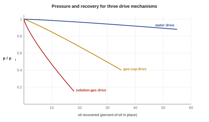
| Drive mechanism | Pressure behavior | Gas-oil ratio | Typical primary recovery |
|---|---|---|---|
| Solution-gas drive | Falls quickly | Rises sharply below the bubble point | 5 to 25 % |
| Gas-cap drive | Falls slowly | Rises as the cap reaches wells | 20 to 40 % |
| Water drive | Stays high | Stays low | 35 to 60 % |
| Gravity drainage | Varies | Low in down-dip wells | Up to 60 % in favorable cases |
When natural energy is weak, engineers add energy. Waterflooding injects water into wells on a pattern so that it sweeps oil toward producing wells while holding up the reservoir pressure; it is the most widely used method of improving recovery in the world. Gas injection maintains pressure in a gas cap or, at high enough pressure, mixes with the oil and reduces its viscosity. Enhanced oil recovery methods such as carbon dioxide flooding, chemical floods and steam injection, covered in PET-430, alter the fluids or rock to free oil that water cannot move.
In the Bakken, waterflooding has not worked well because the rock's permeability is so low that water barely moves through it. Several operators have tested gas injection, using produced gas, to push oil out of the tight matrix in a repeated cycle of injecting and producing, often called huff-and-puff. Results have been mixed, and recovery factors in the play remain mostly in the single digits.
Material balance
Material balance applies conservation of mass to the reservoir as a whole. The volume of fluid withdrawn must equal the expansion of the fluids and rock left behind plus any water that flows in. For a dry gas reservoir with no water influx, the result is especially simple: the ratio of pressure to gas compressibility factor, p/z, falls in a straight line as cumulative gas production increases. Extrapolating that line to zero gives the original gas in place. Engineers plot p/z from shut-in pressure tests against cumulative production, and a straight line confirms both the estimate and the absence of water drive.
For oil reservoirs, the general material balance equation includes terms for oil and solution gas expansion, gas cap expansion, rock and water compressibility and water influx. Fitting it to production and pressure data reveals which drive mechanisms are active and how strong each is. It needs only a few averaged properties, which makes it a useful check on more detailed numerical simulation models that divide the reservoir into thousands of cells.
Decline curve analysis
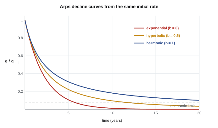
Production from a well or field typically declines with time. In 1945, J. J. Arps described three common shapes. With exponential decline, the rate falls by the same percentage each year. With hyperbolic decline, the percentage drop itself shrinks with time, so the curve flattens. Harmonic decline is a special hyperbolic case. The general form is:
Here \(q_i\) is the initial rate, \(D_i\) the initial decline rate and b the hyperbolic exponent: b = 0 is exponential, 0 < b < 1 hyperbolic and b = 1 harmonic. Integrating the curve to an economic limit, the rate at which the well's revenue no longer covers its operating cost, gives the estimated ultimate recovery (EUR) of the well. Tight oil wells decline very steeply at first, often losing 60 to 70 percent of their initial rate in the first year, and then flatten. Fitting them with b values above 1 matches the early data but would predict unrealistic recovery if extended, so evaluators switch to an exponential tail, typically at a terminal decline of 6 to 10 percent per year.
Worked problem
Ultimate recovery from a decline curve
A new Tamarack Lake field well starts at 900 bbl/d of oil. Ethan fits an exponential decline with D = 0.60 per year in continuous form, as a simple first estimate. The economic limit is 20 bbl/d. How long will the well produce, and what is its ultimate recovery?
Show solution
- For exponential decline, q = q_i·e^(−Dt), so t = ln(q_i/q_ec)/D = ln(900/20)/0.60 = 3.807/0.60 = 6.3 years.
- Cumulative production: N_p = (q_i − q_ec)/D = (900 − 20) bbl/d × 365 d/yr / 0.60 per yr = 535,000 bbl.
Answer: About 6 years and 535,000 bbl. Real Bakken wells decline hyperbolically and produce for decades at low rates, so a hyperbolic fit with an exponential tail gives a longer life; the choice of b is one of the main judgments in a reserve estimate.
Simulation and uncertainty
For large fields and complex decisions, reservoir engineers build numerical simulation models. The reservoir is divided into thousands or millions of grid cells, each assigned porosity, permeability, saturation and pressure from the geological model. The simulator solves the equations of mass conservation and Darcy flow in every cell over time steps, predicting rates, pressures and saturations for any development plan. Engineers adjust the model until it reproduces the field's production and pressure history, a process called history matching, and then use it to compare infill drilling, waterflood patterns or enhanced recovery schemes. PET-420 Reservoir Simulation covers the method.
Every estimate of volumes and recovery is uncertain, and good practice is to express that uncertainty honestly. Engineers vary each input, such as area, thickness, porosity, saturation and recovery factor, across its plausible range, often in a Monte Carlo calculation that samples thousands of combinations, and report the results as low, best and high estimates. Lesson 10 shows how these estimates map onto reserve categories. An engineer who reports a single number without a range invites decisions that are more confident than the data allow.
Common mistakes
MistakeTreating oil in place as recoverable oil.
InsteadMultiply by a recovery factor that reflects the drive mechanism and development plan.
MistakeUsing gross thickness in volumetrics.
InsteadUse net pay, the thickness of rock good enough to contribute.
MistakeExtrapolating a hyperbolic decline with b > 1 forever.
InsteadSwitch to an exponential terminal decline; otherwise recovery is overstated.
MistakeIgnoring water influx in a gas material balance.
InsteadA p/z plot that curves upward suggests water drive and makes the straight-line estimate too high.
Summary and key terms
- Oil in place is A·h·φ(1 − S_w)/B_o; gas in place uses B_g. Recovery factors convert in-place volumes to recoverable volumes.
- Drive mechanisms supply the energy: solution gas, gas cap, water, gravity and compaction, with very different recoveries.
- Waterflooding and gas injection add energy; enhanced recovery changes fluid or rock behavior.
- Material balance treats the reservoir as a tank; for dry gas, p/z falls linearly with cumulative production.
- Arps decline curves, q = q_i/(1 + b·D_i·t)^(1/b), extrapolate production to an economic limit to give EUR.
- Tight oil wells decline steeply and need a terminal exponential decline to avoid overstating reserves.
- Original oil in place
- The total volume of oil in a reservoir before production, at stock-tank conditions.
- Recovery factor
- The fraction of the oil or gas in place that can be produced.
- Drive mechanism
- The natural source of energy that moves fluids to the wells.
- Waterflood
- Injection of water to maintain pressure and sweep oil toward producing wells.
- Material balance
- An accounting of fluids produced, expanded and injected, used to estimate volumes and drive mechanisms.
- Decline curve
- A graph or equation describing how a well's production rate falls with time.
- Estimated ultimate recovery (EUR)
- The total volume a well or field is expected to produce over its life.
Practice problems
Work each problem on paper first, then reveal the answer to check.
A reservoir has A = 640 acres, h = 25 ft, φ = 0.18, S_w = 0.25 and B_o = 1.25. Find N.
Show answer
N = 7,758 × 640 × 25 × 0.18 × 0.75/1.25 = 13.4 million STB.
A gas reservoir started with p/z = 4,000 psia and after producing 20 Bcf has p/z = 3,200 psia. Estimate the original gas in place.
Show answer
p/z fell 800 psia, or 20 percent of 4,000, for 20 Bcf, so G = 20/0.20 = 100 Bcf.
Which drive mechanism would you expect if pressure stays nearly constant while water production rises steadily?
Show answer
A strong water drive.
What does the b exponent in the Arps equation describe?
Show answer
How much the decline rate itself decreases with time: b = 0 is exponential, 0 < b < 1 hyperbolic and b = 1 harmonic.
Lesson quiz · 5 questions
Score 60% or more to complete this lesson.
Create a free account to save your progress, take quizzes and earn a certificate.