
MEC-340 · Lesson 4 of 12 · 23 min
Two-dimensional and numerical conduction
Most of the new transmission main will not sit in a tunnel; it will be buried about 1.2 m deep in the clay soils of Minneapolis. Heat leaving the pipe spreads through the soil in two dimensions on its way to the ground surface, so the one-dimensional resistances of Lesson 2 are no longer enough. The same is true of a steam pipe cast into a concrete encasement under a road, a corner of a valve chamber, or the edge of a floor slab. This lesson presents two tools for multidimensional steady conduction: conduction shape factors, which package known solutions into a resistance, and the finite-difference method, which can solve almost any geometry on a computer.
Two-dimensional steady conduction
With no generation and constant conductivity, steady two-dimensional conduction obeys Laplace's equation:
Exact solutions exist for simple shapes and boundary conditions. The method of separation of variables, applied to a rectangle with one edge at a different temperature from the other three, gives a series of sine and hyperbolic sine terms. Line sources and their images give the field around a buried pipe exactly: the isotherms are circles whose centers lie below the pipe and crowd toward the ground surface. These analytical solutions are elegant but limited, and engineers usually reach for one of two practical tools.
Conduction shape factors
For many common two-dimensional geometries between two isothermal surfaces, the heat rate can be written as
where \(S\), the conduction shape factor, has units of length and depends only on the geometry. Shape factors are tabulated in heat transfer texts for dozens of configurations. A few that appear at Northgate:
| Configuration | Shape factor S | Condition |
|---|---|---|
| Horizontal cylinder of length L buried at depth z (to center) in a semi-infinite medium | \(\frac{2\pi L}{\cosh^{-1}(2z/D)}\) | \(L \gg D\) |
| Same, approximate form | \(\frac{2\pi L}{\ln(4z/D)}\) | \(z > 3D/2\) |
| Cylinder centered in a square solid of side w | \(\frac{2\pi L}{\ln(1.08\,w/D)}\) | \(w > D\) |
| Two parallel cylinders, center spacing s, in an infinite medium | \(\frac{2\pi L}{\cosh^{-1}\!\big(\frac{4s^2 - D_1^2 - D_2^2}{2D_1D_2}\big)}\) | \(L \gg D_1, D_2, s\) |
| Edge of two adjoining walls of thickness L | \(0.54\,D\) | D = wall length |
| Corner of three walls of thickness L | \(0.15\,L\) | Each wall much larger than L |
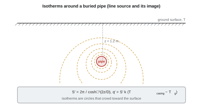
For a buried pipe, the ground surface is treated as an isotherm at the surface temperature, which in a Minneapolis January is well below freezing. The soil resistance is in series with the pipe's own resistance from Lesson 2, so the heat loss follows from the total. Soil conductivity varies widely: about 0.3 W/m·K for dry sand, 1 to 1.5 W/m·K for moist clay, and more for saturated or frozen soils, since ice conducts about four times better than water. Utilities often assume a single design value and check the sensitivity.
# Two-dimensional conduction: shape factors and a finite-difference model
import math

# 1. Shape factor for a buried pre-insulated pipe (per 1 m length), in series with the pipe's own resistance
k_soil, z, Dc = 1.2, 1.2, 0.315           # moist clay (W/m.K), depth to pipe axis, casing OD (m)
S = 2 * math.pi / math.acosh(2 * z / Dc)  # shape factor per 1 m length of pipe
R_soil, R_pipe = 1 / (S * k_soil), 1.965  # m.K/W; the pipe value (foam + casing) comes from Lesson 2
T_w, T_g = 110.0, -5.0                    # supply water; ground surface in midwinter
q = (T_w - T_g) / (R_pipe + R_soil)
print(f"buried pipe: S' = {S:.3f}, soil R' = {R_soil:.3f} m.K/W, loss {q:.1f} W/m, casing at {T_g + q*R_soil:.1f} C")
print(f"  ln(4z/D) approximation gives S' = {2*math.pi/math.log(4*z/Dc):.3f}")

# 2. Finite differences: a bare steam pipe cast in a square concrete encasement.
#    One quarter of the section is solved; x = 0 and y = 0 are symmetry lines.
def encasement(N, D=0.20, w=0.60, T_in=170.0, T_out=10.0, k=1.4, omega=1.8, tol=1e-6):
    dx = (w / 2) / N
    T = [list([T_out] * (N + 1)) for _ in range(N + 1)]
    fixed = [list([False] * (N + 1)) for _ in range(N + 1)]
    for j in range(N + 1):
        for i in range(N + 1):
            if i == N or j == N: fixed[j][i] = True                         # outer face of the concrete
            elif math.hypot(i * dx, j * dx) <= D / 2 + 1e-12:
                T[j][i], fixed[j][i] = T_in, True                           # inside the pipe
    for sweep in range(20000):
        change = 0.0
        for j in range(N):
            for i in range(N):
                if fixed[j][i]: continue
                W = T[j][i - 1] if i > 0 else T[j][1]                       # mirror across x = 0
                Sn = T[j - 1][i] if j > 0 else T[1][i]                      # mirror across y = 0
                new = 0.25 * (W + T[j][i + 1] + Sn + T[j + 1][i])
                d = new - T[j][i]; T[j][i] += omega * d; change = max(change, abs(d))
        if change < tol: break
    # heat leaving through the outer face x = w/2 of the quarter (the y-face carries the same by symmetry)
    q_quarter = 0.0
    for j in range(N):
        wgt = 0.5 if j == 0 else 1.0
        q_quarter += wgt * k * (T[j][N - 1] - T[j][N])
    return 4 * 2 * q_quarter, sweep, T[0][N // 2]

D, w, k = 0.20, 0.60, 1.4
S_formula = 2 * math.pi / math.log(1.08 * w / D)
print(f"\nencased pipe, shape-factor formula: S' = {S_formula:.3f}, q' = {S_formula*k*160:.0f} W/m")
for N in (15, 30, 60):
    qn, sw, Tmid = encasement(N)
print(f"grid {N:2d} x {N:2d} (dx = {300/N:4.1f} mm): {sw:4d} sweeps, q' = {qn:6.0f} W/m, T halfway out = {Tmid:6.1f} C")buried pipe: S' = 2.310, soil R' = 0.361 m.K/W, loss 49.4 W/m, casing at 12.8 C ln(4z/D) approximation gives S' = 2.307 encased pipe, shape-factor formula: S' = 5.345, q' = 1197 W/m grid 15 x 15 (dx = 20.0 mm): 79 sweeps, q' = 1155 W/m, T halfway out = 119.3 C grid 30 x 30 (dx = 10.0 mm): 145 sweeps, q' = 1170 W/m, T halfway out = 111.3 C grid 60 x 60 (dx = 5.0 mm): 633 sweeps, q' = 1181 W/m, T halfway out = 112.4 C
Worked problem
The buried transmission main
The pre-insulated pipe of Lesson 2 (casing diameter 315 mm, pipe resistance foam plus casing 1.965 m·K/W) is buried with its center 1.2 m deep in clay with k = 1.2 W/m·K. Water is at 110 °C and the ground surface at −5 °C. Find the heat loss per meter and the casing temperature.
Show solution
- Shape factor: \(S' = 2\pi/\cosh^{-1}(2 \times 1.2/0.315) = 2\pi/\cosh^{-1}(7.62) = 2.310\).
- Soil resistance: \(R'_{\text{soil}} = 1/(2.310 \times 1.2) = 0.361\) m·K/W.
- Total: \(R' = 1.965 + 0.361 = 2.326\) m·K/W (water film and steel negligible).
- \[q' = \frac{110 - (-5)}{2.326} = 49.4\ \text{W/m}, \qquad T_{\text{casing}} = -5 + 49.4(0.361) = 12.8\ ^\circ\text{C}\]
Answer: The soil adds only about 16 percent to the resistance, because the foam already dominates. The loss is a little higher than in the tunnel, mainly because the ground surface is colder than the tunnel air. The approximate shape factor, \(2\pi/\ln(4z/D)\), gives 2.307, almost identical, since the pipe is buried more than seven diameters deep.
A real district system lays the supply and return pipes side by side in the same trench. Each pipe warms the soil around the other, so the supply loses a little less heat and the return a little more than if each were alone. The two-cylinder shape factor in the table, combined with the superposition of their fields, handles this interaction; for pipes spaced one or two diameters apart the correction is typically a few percent. Some systems use twin pipes, with supply and return inside one casing, which reduces the total loss further.
The finite-difference method
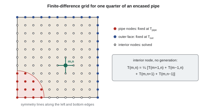
When no shape factor exists, the temperature field must be computed. The finite-difference method replaces the continuous region with a grid of nodes spaced \(\Delta x\) apart and replaces the derivatives in Laplace's equation with differences between neighboring nodes. For a square grid and an interior node \((m, n)\), the second derivatives become
and similarly in \(y\). Substituting into Laplace's equation gives the simplest and most famous result in numerical heat transfer: each interior node's temperature is the average of its four neighbors,
The same equation follows from an energy balance on the small square of material around the node: the heat conducted in from each neighbor, \(k\,\Delta y\,(T_{\text{nb}} - T_{m,n})/\Delta x\) per unit depth, must sum to zero. The energy-balance view is the better one in practice, because it extends directly to nodes on boundaries, at corners, on convective surfaces and in regions with generation. A node on a symmetry line, for example, is treated as if a mirror-image node lay beyond the line, and a node on a convective surface balances conduction from its neighbors against \(h\,\Delta x\,(T_\infty - T_{m,n})\).
Solving the equations
A grid of \(N\) unknown nodes gives \(N\) linear equations. For small grids they can be solved directly by matrix methods. For large grids, iterative methods are simpler and use little memory. In the Gauss-Seidel method, each node is updated in turn from the latest values of its neighbors, and sweeps through the grid are repeated until the largest change falls below a tolerance. Over-relaxation, which overshoots each update by a factor \(\omega\) between 1 and 2, speeds convergence greatly. After convergence, the heat rate is found by summing the conduction across a boundary, and the result should be checked by refining the grid: if halving \(\Delta x\) changes the heat rate by less than the accuracy needed, the grid is fine enough.
Worked problem
A steam pipe in a concrete encasement
Where the steam line crosses a road it is a bare pipe of 200 mm outside diameter cast into a square concrete encasement 0.6 m on a side (k = 1.4 W/m·K). The pipe surface is at 170 °C and the outer faces of the concrete at 10 °C. Find the heat loss per meter by shape factor and by finite differences.
Show solution
- Shape factor: \(S' = 2\pi/\ln(1.08 \times 0.6/0.2) = 2\pi/\ln 3.24 = 5.345\).
- \(q' = 5.345 \times 1.4 \times 160 = 1197\) W/m.
- Finite differences on one quarter of the section with Gauss-Seidel over-relaxation: 15 × 15 grid, 1155 W/m; 30 × 30, 1170 W/m; 60 × 60, 1181 W/m.
Answer: The numerical result approaches the shape-factor value as the grid is refined; the remaining difference comes partly from the staircase representation of the round pipe on a square grid and partly from the shape factor itself, which is an approximation. A loss of about 1.2 kW per meter is enormous compared with the 43 W/m of the pre-insulated pipe, which is why encased bare steam lines are being replaced throughout the industry.
Commercial finite-element and finite-volume software applies the same principles to irregular meshes, three dimensions, variable properties and coupled fluid flow. The finite-difference method remains valuable for understanding what such software does and for checking it: a simple model that reproduces a known shape factor builds confidence that a more complex model has been set up correctly.
In the United States, frost depth for foundations and buried services is set by local codes; in the Minneapolis area, footing depths of about 42 inches (1.07 m) are common, with deeper requirements farther north in Minnesota. Buried district heating pipes warm the soil above them, and snow melting faster over a line is a quick field check on its insulation. In US units, the buried main's 49.4 W/m is about 51 Btu/h per foot of pipe.
Common mistakes
MistakeApplying a shape factor outside its conditions.
InsteadCheck the geometric limits, such as L much greater than D or z greater than 3D/2.
MistakeForgetting the pipe's own resistance in series with the soil.
InsteadThe foam usually dominates; add the soil shape-factor resistance to it.
MistakeStopping Gauss-Seidel iterations too early.
InsteadUse a tight tolerance and confirm the heat rate has converged.
MistakeTrusting a single grid.
InsteadRefine the grid and check that the answer changes little.
MistakeTreating a symmetry line as a fixed-temperature boundary.
InsteadA symmetry line is adiabatic; use mirror-image nodes.
Summary and key terms
- Steady two-dimensional conduction without generation obeys Laplace's equation.
- Shape factors give q = Sk(T₁ − T₂) for standard geometries; R = 1/(Sk).
- The buried main loses about 49 W/m; the soil adds only about 16 percent to the resistance.
- Finite differences make each interior node the average of its four neighbors.
- Energy balances on nodes handle boundaries, symmetry, convection and generation.
- Gauss-Seidel with over-relaxation solves large grids; grid refinement checks the answer.
- Laplace's equation
- The steady conduction equation with no generation, ∇²T = 0.
- Conduction shape factor
- A geometric factor S such that q = Sk ΔT for two-dimensional conduction.
- Semi-infinite medium
- A body bounded by one plane surface and extending indefinitely, used to model the ground.
- Finite-difference method
- A numerical method that replaces derivatives with differences between grid nodes.
- Node
- A grid point at which the temperature is computed.
- Gauss-Seidel iteration
- An iterative method that updates each node from the latest neighboring values.
- Over-relaxation
- Multiplying each Gauss-Seidel correction by a factor between 1 and 2 to speed convergence.
- Grid independence
- The condition in which refining the grid no longer changes the result significantly.
- Symmetry line
- A line across which the temperature field is mirrored, with no heat crossing it.
Practice problems
Work each problem on paper first, then reveal the answer to check.
Find the shape factor per meter for a pipe of 0.3 m diameter buried 0.9 m deep (to its center).
Show answer
2π/cosh⁻¹(6) = 2.53.
In the buried-main example, change the soil conductivity to 0.5 W/m·K (dry soil). Find the new loss.
Show answer
Soil R′ = 0.866; total 2.831 m·K/W; q′ ≈ 40.6 W/m.
Write the finite-difference equation for a node on an adiabatic boundary at the left edge of a grid.
Show answer
T_m,n = ¼(2T_m+1,n + T_m,n+1 + T_m,n−1).
An interior node's four neighbors are at 40, 50, 60 and 70 °C. What is its temperature?
Show answer
55 °C.
In the program, enlarge the encasement to w = 1.0 m. What does the shape factor give?
Show answer
S′ = 2π/ln(5.4) = 3.72; q′ ≈ 835 W/m.
Why does refining the grid change the encased-pipe result?
Show answer
Finer grids represent the round pipe and the temperature gradients more accurately.
Lesson quiz · 5 questions
Score 60% or more to complete this lesson.
Create a free account to save your progress, take quizzes and earn a certificate.