
ELE-250 · Lesson 7 of 12 · 23 min
The continuous-time Fourier transform
The Fourier series handles periodic signals, but many of the signals Amara cares about are not periodic. A single tick of the locator tone, the burst of noise from a passing truck and a speech message announcing the street name all start and stop. The Fourier transform extends frequency analysis to such signals. Instead of a set of lines at harmonic frequencies, a non-periodic signal has a continuous spectrum that spreads its content over a range of frequencies. The transform turns convolution into multiplication, which is why it is the main working tool for filters, communication systems and audio processing, and it explains a basic trade-off of signal design: the shorter a signal is in time, the wider it is in frequency.
From series to transform
Imagine a pulse repeated every T₀ seconds and let T₀ grow. The harmonics, spaced ω₀ = 2π/T₀ apart, crowd closer together, and each coefficient c_k shrinks in proportion to 1/T₀ because the pulse occupies a smaller fraction of each period. In the limit of a single pulse, the spacing becomes infinitesimal, the lines merge into a continuous curve, and the product T₀c_k becomes a function of the continuous frequency ω. That function is the Fourier transform:
The first integral is the analysis equation, which measures how much of each frequency the signal contains; the second is the synthesis equation, which rebuilds the signal from its frequency content. X(jω) is a density: |X(jω)|² dω/2π is the energy in a small band of width dω. The notation x(t) ↔ X(jω) says the two are a transform pair. Some books use the ordinary frequency f in hertz, with ω = 2πf, which removes the 1/2π from the inverse; both conventions appear in practice, so always check which one a table uses.
Three essential pairs
The rectangular pulse of height 1 and width τ, centered at t = 0, transforms to a sinc-shaped spectrum. Integrating e^(−jωt) from −τ/2 to τ/2 gives
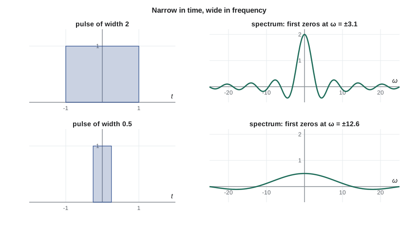
The spectrum has its peak value τ, the pulse's area, at ω = 0, and it first reaches zero at ω = 2π/τ, which is f = 1/τ in hertz. A 1 ms pulse has its first spectral null at 1 kHz; a 0.1 ms pulse at 10 kHz. Most of the energy lies in the main lobe between the first nulls, so the bandwidth of a pulse is roughly the inverse of its duration.
The decaying exponential e^(−at)u(t), with a > 0, transforms to 1/(a + jω), whose magnitude 1/√(a² + ω²) falls off smoothly as frequency rises. The unit impulse transforms to 1 at every frequency: an infinitely short event contains all frequencies equally, which is why a sharp click excites every resonance of a room or a structure. In the other direction, a constant contains only zero frequency, and its transform is an impulse, 2πδ(ω).
Worked problem
Spectrum of a short pulse
The tachometer's conditioning circuit produces 0.2 ms pulses of height 5 V. Find the transform, the value at zero frequency and the frequency of the first null.
Show solution
- Scale the rect pair by 5 and use τ = 0.2 ms.
- \[X(j\omega) = 5\tau\,\frac{\sin(\omega\tau/2)}{\omega\tau/2} = 10^{-3}\,\frac{\sin(10^{-4}\omega)}{10^{-4}\omega}\ \text{V·s}\]
- At zero frequency the sinc equals 1, so X(0) is the pulse's area.
- \[X(0) = 5 \times 0.2 \times 10^{-3} = 10^{-3}\ \text{V·s}\]
- The first null is where ωτ/2 = π.
Answer: X(0) = 1 mV·s and the first null is at f = 1/τ = 5 kHz. The pulse's energy is concentrated below about 5 kHz, which tells Daniel how much bandwidth the tachometer input stage needs to keep the pulse shape recognizable.
Properties
A handful of properties lets you find most transforms from a few known pairs instead of integrating. Linearity: a sum of signals transforms to the sum of their transforms. Time shift: delaying a signal by t₀ multiplies its transform by e^(−jωt₀), which changes only the phase, not the magnitude, so a delayed tick has the same spectrum magnitude as an early one. Time scaling: compressing a signal in time by a factor a stretches its spectrum by a, x(at) ↔ (1/|a|)X(jω/a), the formal version of the duration–bandwidth trade-off. Conjugate symmetry: for a real signal X(−jω) = X(jω)*, so the magnitude spectrum is even and only positive frequencies need to be plotted.
Two properties matter more than the rest. The convolution property says that convolving in time becomes multiplying in frequency:
An LTI system therefore multiplies the input spectrum by its frequency response, H(jω), the Fourier transform of its impulse response. That is the whole idea of filtering, and lesson 8 builds on it. The dual modulation property says that multiplying in time becomes convolving in frequency, scaled by 1/2π. Multiplying a signal by cos(ω₀t) shifts its spectrum up and down by ω₀:
This is how AM radio moves audio up to a carrier frequency, and it explains the spectrum of a tone burst, as the next example shows. Differentiation in time multiplies the transform by jω, which is why differentiating a signal emphasizes its high frequencies and why the derivative of noisy data is noisier still. Parseval's theorem gives the energy in either domain: ∫|x(t)|²dt = (1/2π)∫|X(jω)|²dω.
| Signal x(t) | Transform X(jω) | Comment |
|---|---|---|
| δ(t) | 1 | All frequencies equally |
| 1 | 2πδ(ω) | DC only |
| e^(−at)u(t), a > 0 | 1/(a + jω) | RC-type decay |
| rect(t/τ) | τ sin(ωτ/2)/(ωτ/2) | First null at f = 1/τ |
| cos(ω₀t) | π[δ(ω − ω₀) + δ(ω + ω₀)] | Two lines at ±ω₀ |
| x(t − t₀) | e^(−jωt₀)X(jω) | Delay changes phase only |
| x(at) | (1/|a|)X(jω/a) | Compress in time, stretch in frequency |
| x(t) * h(t) | X(jω)H(jω) | Convolution becomes multiplication |
| x(t)cos(ω₀t) | ½X(j(ω − ω₀)) + ½X(j(ω + ω₀)) | Modulation shifts the spectrum |
| dx/dt | jωX(jω) | Emphasizes high frequencies |
Worked problem
Spectrum of a locator-tone tick
Each locator tick is an 880 Hz tone switched on for 20 ms: x(t) = rect(t/τ)cos(ω₀t) with τ = 20 ms and ω₀ = 2π(880). Describe its spectrum.
Show solution
- The rect pulse alone has a sinc spectrum centered at zero with first nulls at ±1/τ = ±50 Hz.
- \[\text{rect}(t/\tau) \;\Longleftrightarrow\; \tau\,\frac{\sin(\omega\tau/2)}{\omega\tau/2}\]
- Multiplying by cos(ω₀t) shifts half of that spectrum to +880 Hz and half to −880 Hz.
- \[X(j\omega) = \frac{\tau}{2}\,\frac{\sin\big((\omega-\omega_0)\tau/2\big)}{(\omega-\omega_0)\tau/2} + \frac{\tau}{2}\,\frac{\sin\big((\omega+\omega_0)\tau/2\big)}{(\omega+\omega_0)\tau/2}\]
- At positive frequencies, the main lobe runs from 880 − 50 = 830 Hz to 880 + 50 = 930 Hz.
Answer: The tick's energy is concentrated in a band about 100 Hz wide centered on 880 Hz, with side lobes that fall off slowly because the tone switches on and off abruptly. A shorter tick would spread wider; switching the tone on and off with gentle ramps instead of hard edges would shrink the side lobes.
Periodic signals and the transform
The Fourier transform also covers periodic signals, which ties it back to lesson 6. A periodic signal with Fourier coefficients c_k has a transform made of impulses at the harmonic frequencies: X(jω) = Σ 2πc_k δ(ω − kω₀). Each line of the line spectrum becomes an impulse whose area is 2π times the coefficient. The cosine entry in the table is the simplest case, with c_{±1} = ½. Writing periodic and non-periodic signals in one framework means a single set of tools handles a signal that is partly both, such as the steady 60 Hz hum, which is a pair of impulses at ±60 Hz, plus the occasional truck, which is a continuous spread. It also shows something useful about the square wave from lesson 6: its coefficients c_k = d·sin(πkd)/(πkd) are samples of the transform of a single pulse, taken at the harmonic frequencies and divided by the period. Repeating a signal in time samples its spectrum in frequency, a fact that returns in lesson 9 with the roles of time and frequency swapped.
The frequency response is a transform
Because the output spectrum is X(jω)H(jω), the frequency response H(jω) is simply the Fourier transform of the impulse response. For the RC low-pass filter, h(t) = (1/RC)e^(−t/RC)u(t), and the table gives H(jω) = 1/(1 + jωRC). The magnitude starts at 1 at DC and falls as frequency rises, which is exactly what a low-pass filter should do. There are therefore two equivalent ways to find a filter's output: convolve the input with h(t) in time, or multiply the spectra and transform back. For simple signals the second is often far easier, and for long signals on a computer the fast Fourier transform of lesson 10 makes it far faster.
Duration, bandwidth and uncertainty
The pairs above share a pattern: whatever shape a signal has, squeezing it in time spreads it in frequency. No signal can be both very short and very narrow in frequency. Defined carefully with root-mean-square widths, the product of duration and bandwidth has a minimum value that only a Gaussian pulse achieves. Engineers meet this limit everywhere. A radar that wants to resolve close targets needs short pulses and therefore wide bandwidth; a radio channel with narrow bandwidth cannot carry fast symbols; and a noise meter that wants to tell 880 Hz from 900 Hz must listen for tens of milliseconds. For the pedestrian signal it means the locator tick cannot be both very short and very pure in pitch.
import math, cmath

def ft(x, t, w):
    """Approximate X(jw) = integral x(t) exp(-j w t) dt with a Riemann sum."""
    dt = t[1] - t[0]
    return sum(xv * cmath.exp(-1j * w * tv) for xv, tv in zip(x, t)) * dt

tau, f0 = 20e-3, 880.0
dt = 1e-5
t = [-tau / 2 + n * dt for n in range(int(tau / dt))]
x = [math.cos(2 * math.pi * f0 * tv) for tv in t]

def exact(f):
    def half(u):
        return tau / 2 if abs(u) < 1e-12 else tau / 2 * math.sin(u * tau / 2) / (u * tau / 2)
    w = 2 * math.pi * f
    return half(w - 2 * math.pi * f0) + half(w + 2 * math.pi * f0)

for f in (0, 800, 830, 860, 880, 900, 930, 1000):
    num = abs(ft(x, t, 2 * math.pi * f))
print(f"{f:5d} Hz: |X| numeric {num*1e3:7.3f} ms exact {abs(exact(f))*1e3:7.3f} ms")0 Hz: |X| numeric 0.346 ms exact 0.344 ms 800 Hz: |X| numeric 1.985 ms exact 1.982 ms 830 Hz: |X| numeric 0.056 ms exact 0.055 ms 860 Hz: |X| numeric 7.624 ms exact 7.622 ms 880 Hz: |X| numeric 9.946 ms exact 9.947 ms 900 Hz: |X| numeric 7.481 ms exact 7.483 ms 930 Hz: |X| numeric 0.053 ms exact 0.052 ms 1000 Hz: |X| numeric 1.178 ms exact 1.181 ms
The numerical and exact magnitudes agree to within a fraction of a percent. The peak at 880 Hz is very nearly τ/2 = 10 ms; the small shortfall comes from the tail of the mirror-image lobe centered at −880 Hz, which overlaps slightly. The near-zeros at 830 and 930 Hz mark the ends of the main lobe, and at 860 and 900 Hz, 20 Hz from the center, the magnitude has already dropped to about 75 % of the peak. Content at 800 and 1,000 Hz comes from the side lobes. When Amara's noise detector listens for traffic noise, she excludes a band around 880 Hz wide enough to hold the tick's main lobe, so the detector does not mistake the signal's own tick for street noise.
Common mistakes
MistakeMixing up angular frequency ω and frequency f.
Insteadω = 2πf; the rect pair's first null is at ω = 2π/τ, which is f = 1/τ.
MistakeThinking a time delay changes the magnitude spectrum.
InsteadA delay multiplies X by e^(−jωt₀), whose magnitude is 1; only the phase changes.
MistakeExpecting a short tick to have a pure pitch.
InsteadDuration and bandwidth trade off; a 20 ms tick spreads over about 100 Hz.
MistakeForgetting the 1/2π in the inverse transform or in Parseval's theorem.
InsteadWith ω in rad/s, both carry 1/2π; with f in hertz, neither does.
MistakePlotting only positive frequencies of a complex-valued signal.
InsteadConjugate symmetry, and hence a mirror-image magnitude, holds only for real signals.
Summary and key terms
- The Fourier transform X(jω) = ∫x(t)e^(−jωt)dt gives a continuous spectrum for non-periodic signals; the inverse rebuilds the signal.
- A rectangular pulse of width τ has a sinc spectrum with first nulls at f = ±1/τ; an impulse contains all frequencies equally.
- Delay changes only phase, time compression stretches the spectrum, and real signals have even magnitude spectra.
- Convolution in time becomes multiplication in frequency: Y(jω) = X(jω)H(jω).
- Multiplication by cos(ω₀t) shifts a spectrum to ±ω₀, which explains tone bursts and amplitude modulation.
- Short signals are wide in frequency and narrow-band signals are long in time.
- Fourier transform
- X(jω) = ∫x(t)e^(−jωt)dt, the frequency-domain description of a non-periodic signal.
- Spectrum
- The magnitude and phase of a signal’s Fourier transform as functions of frequency.
- Sinc function
- sin(u)/u, the shape of the Fourier transform of a rectangular pulse.
- Modulation property
- Multiplying by cos(ω₀t) shifts the spectrum up and down by ω₀.
- Bandwidth
- The range of frequencies that holds most of a signal’s energy.
- Conjugate symmetry
- The property X(−jω) = X(jω)* of the transform of a real signal.
Practice problems
Work each problem on paper first, then reveal the answer to check.
Find the transform of 3e^(−2t)u(t).
Show answer
3/(2 + jω).
A pulse has transform X(jω). What is the transform of the same pulse delayed by 5 ms?
Show answer
e^(−j0.005ω)X(jω); same magnitude, extra linear phase.
A 0.5 ms rectangular pulse has its first spectral null where?
Show answer
At 2 kHz.
What is the transform of x(2t) if x(t) ↔ X(jω)?
Show answer
½X(jω/2): half as tall and twice as wide.
A 1 kHz tone is switched on for 5 ms. How wide is the main lobe of its spectrum?
Show answer
From 800 to 1,200 Hz, 400 Hz wide, since 1/τ = 200 Hz.
An LTI system has H(jω) = 1/(1 + jω/1000). What is its impulse response?
Show answer
h(t) = 1000e^(−1000t)u(t).
Lesson quiz · 5 questions
Score 60% or more to complete this lesson.
Create a free account to save your progress, take quizzes and earn a certificate.