
ELE-250 · Lesson 11 of 12 · 23 min
The Laplace transform
The Fourier transform describes signals as sums of sinusoids that last forever, which makes it ideal for steady-state filtering but awkward for three jobs engineers face constantly: signals that grow, systems that start with stored energy, and questions of stability. The Laplace transform handles all three. It replaces the pure oscillation e^(jωt) with the more general exponential e^(st), where s = σ + jω can decay or grow as well as oscillate. In return for one more dimension, it turns differential equations into algebra, turns convolution into multiplication, and lets an engineer judge a system's stability by looking at where a few numbers, its poles, sit on a plane. The Cedarline team uses it to analyze the second-order anti-aliasing stage and the locator tone's automatic volume loop.
Definition and region of convergence
The Laplace transform of a signal x(t) is
The factor e^(−σt) damps the signal, so the integral can converge even for signals, such as a growing exponential, whose Fourier transform does not exist. It converges only for some values of s, and that set, the region of convergence (ROC), is part of the answer. For the causal signal e^(−at)u(t), the integral gives 1/(s + a) when Re{s} > −a. For causal signals the ROC is always everything to the right of some vertical line in the s-plane.
Most engineering work uses the unilateral transform, which integrates from t = 0⁻, just before zero, to infinity. It assumes signals start at t = 0, which suits switching events and lets initial conditions enter the calculation naturally. When the ROC includes the imaginary axis, setting s = jω in X(s) gives the Fourier transform. The Laplace transform therefore contains the frequency response as a special case: H(jω) is H(s) evaluated along the imaginary axis.
| x(t), for t ≥ 0 | X(s) | ROC |
|---|---|---|
| δ(t) | 1 | All s |
| u(t) | 1/s | Re{s} > 0 |
| t·u(t) | 1/s² | Re{s} > 0 |
| e^(−at)u(t) | 1/(s + a) | Re{s} > −a |
| cos(ω₀t)u(t) | s/(s² + ω₀²) | Re{s} > 0 |
| sin(ω₀t)u(t) | ω₀/(s² + ω₀²) | Re{s} > 0 |
| e^(−at)cos(ω₀t)u(t) | (s + a)/((s + a)² + ω₀²) | Re{s} > −a |
| e^(−at)sin(ω₀t)u(t) | ω₀/((s + a)² + ω₀²) | Re{s} > −a |
Properties that do the work
Linearity and the time-shift property, x(t − t₀)u(t − t₀) ↔ e^(−st₀)X(s), work as for the Fourier transform. Multiplying by an exponential shifts in s: e^(−at)x(t) ↔ X(s + a), which is how the damped sinusoids in the table follow from the plain ones. Convolution again becomes multiplication, x(t) * h(t) ↔ X(s)H(s).
The differentiation property is what turns calculus into algebra:
Each derivative becomes a multiplication by s, and the initial values appear automatically. Integration from 0 to t becomes division by s. Two limit theorems are handy for checking results: the initial value theorem, x(0⁺) = lim sX(s) as s → ∞, and the final value theorem, x(∞) = lim sX(s) as s → 0, which applies only when the final value exists, meaning all poles of sX(s) lie strictly in the left half-plane.
Transfer functions, poles and zeros
Taking the Laplace transform of a linear differential equation with zero initial conditions turns every d/dt into s. The ratio of output to input transforms is the transfer function, H(s) = Y(s)/X(s), which is also the Laplace transform of the impulse response. For the RC filter, RC dy/dt + y = x becomes (RCs + 1)Y(s) = X(s), so H(s) = 1/(1 + sRC). In general, H(s) is a ratio of polynomials in s,
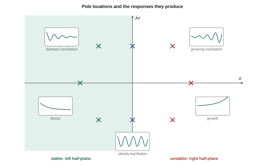
The roots z_i of the numerator are the zeros, where H(s) = 0, and the roots p_i of the denominator are the poles, where H(s) becomes infinite. The poles are the roots of the characteristic equation from lesson 5. Plotting zeros as circles and poles as crosses on the s-plane gives a pole-zero map, and that small picture says almost everything about the system.
Poles and the natural response
Each pole contributes a term to the impulse response. A real pole at s = −a gives e^(−at), which decays if a > 0. A complex-conjugate pair at s = −σ ± jω_d gives a damped sinusoid e^(−σt)cos(ω_dt + φ), oscillating at ω_d and decaying at rate σ. A pole on the imaginary axis gives an oscillation that neither grows nor decays, and a pole in the right half-plane gives a term that grows without limit. The rule for stability follows directly: a causal LTI system is BIBO stable if and only if all its poles lie strictly in the left half of the s-plane. The further left a pole is, the faster its term dies; the closer a complex pair is to the imaginary axis compared with its distance from the real axis, the more lightly damped the ringing.
Worked problem
Poles of a second-order Butterworth stage
Each of the two stages in Amara's fourth-order anti-aliasing filter is a second-order section. A second-order Butterworth low-pass filter with corner ω_c has H(s) = ω_c²/(s² + √2 ω_c s + ω_c²). Find the poles for f_c = 2 kHz and describe its step response.
Show solution
- The poles are the roots of s² + √2 ω_c s + ω_c² = 0.
- \[s = \frac{-\sqrt{2}\,\omega_c \pm \sqrt{2\omega_c^2 - 4\omega_c^2}}{2} = \omega_c\Big(-\frac{1}{\sqrt{2}} \pm j\frac{1}{\sqrt{2}}\Big)\]
- With ω_c = 2π(2000) ≈ 12,570 rad/s:
- \[s \approx -8{,}886 \pm j\,8{,}886\ \text{rad/s}\]
- Comparing with s² + 2ζω_n s + ω_n², the natural frequency is ω_n = ω_c and the damping ratio is ζ = 1/√2 ≈ 0.707.
Answer: The poles sit at 45° from the negative real axis, at radius ω_c. The step response overshoots by about 4 % and settles within roughly 0.5 ms, fast compared with the 32 ms blocks the noise detector analyzes.
Inverse transforms by partial fractions
To get back to time, expand a rational X(s) into a sum of simple terms, one per pole, and read each term's inverse from the table. For distinct poles,
so x(t) = Σ r_i e^(p_i t) for t ≥ 0. The coefficients r_i are the residues. Complex poles come in conjugate pairs with conjugate residues, and each pair combines into a real damped sinusoid. Repeated poles need extra terms of the form t^k e^(pt). This is the systematic version of finding natural and forced responses in lesson 5: the poles of H give the natural terms and the poles of X give the forced terms.
Worked problem
Solving a circuit with an initial condition
Use the Laplace transform to find the RC filter's output when RC = 0.16 ms, the input is a 1.65 V step at t = 0 and the capacitor starts at 0.4 V, the situation from lesson 5.
Show solution
- Transform RC dy/dt + y = x, keeping the initial value. With τ = RC:
- \[\tau\big(sY(s) - 0.4\big) + Y(s) = \frac{1.65}{s} \quad\Rightarrow\quad Y(s) = \frac{1.65}{s(1 + \tau s)} + \frac{0.4\,\tau}{1 + \tau s}\]
- Expand the first term in partial fractions: 1.65/(s(1 + τs)) = 1.65/s − 1.65/(s + 1/τ). The second term is 0.4/(s + 1/τ).
- \[Y(s) = \frac{1.65}{s} - \frac{1.25}{s + 1/\tau}\]
- Invert term by term.
Answer: y(t) = 1.65 − 1.25e^(−t/0.16 ms) V for t ≥ 0, the same answer lesson 5 found by the classical method, but with the initial condition handled automatically by the algebra.
Feedback and stability
The locator tone's automatic volume control measures the noise level, compares it with a target and adjusts the speaker gain. If its controller has transfer function G(s) and the loop gain is K, the closed-loop transfer function is KG(s)/(1 + KG(s)), and its poles are the roots of 1 + KG(s) = 0. Raising K makes the loop respond faster, but it also moves the closed-loop poles. Suppose the level detector and the loudness smoothing together give G(s) = 1/((1 + 0.1s)(1 + 0.02s)), two real poles at −10 and −50 rad/s. With low gain the closed-loop poles stay on the real axis and the volume changes smoothly. As K rises they meet and split into a complex pair, the response starts to overshoot, and the volume swings up and down after a truck passes. This two-pole loop never becomes unstable, but adding the extra delay of a 32 ms analysis block does, at high enough gain, which is why Daniel limits the loop gain and why ELE-390 is devoted to designing such loops.
import cmath, math

def roots2(a, b, c):
    d = cmath.sqrt(b * b - 4 * a * c)
    return (-b + d) / (2 * a), (-b - d) / (2 * a)

wc = 2 * math.pi * 2000
p1, p2 = roots2(1, math.sqrt(2) * wc, wc * wc)
print(f"Butterworth poles: {p1.real:.0f} {p1.imag:+.0f}j and {p2.real:.0f} {p2.imag:+.0f}j rad/s")
zeta = -p1.real / abs(p1)
print(f"damping ratio {zeta:.3f}, overshoot {100*math.exp(-math.pi*zeta/math.sqrt(1-zeta**2)):.1f} %")

# Closed-loop poles of K*G/(1+K*G), G = 1/((1+0.1s)(1+0.02s)) -> 0.002 s^2 + 0.12 s + (1 + K) = 0
for K in (0.5, 1, 4, 10, 40, 160):
    q1, q2 = roots2(0.002, 0.12, 1 + K)
    z = -q1.real / abs(q1)
    kind = "real" if abs(q1.imag) < 1e-9 else f"complex, zeta = {z:.2f}"
    print(f"K = {K:5.1f}: poles {q1.real:7.1f}{q1.imag:+8.1f}j, {q2.real:7.1f}{q2.imag:+8.1f}j  ({kind})")

# Step response of the RC example from residues: y = 1.65 - 1.25 exp(-t/tau)
tau = 0.16e-3
for t in (0.0, 0.16e-3, 0.8e-3):
print(f"t = {t*1e3:.2f} ms: y = {1.65 - 1.25*math.exp(-t/tau):.3f} V")Butterworth poles: -8886 +8886j and -8886 -8886j rad/s damping ratio 0.707, overshoot 4.3 % K = 0.5: poles -17.8 +0.0j, -42.2 +0.0j (real) K = 1.0: poles -30.0 +10.0j, -30.0 -10.0j (complex, zeta = 0.95) K = 4.0: poles -30.0 +40.0j, -30.0 -40.0j (complex, zeta = 0.60) K = 10.0: poles -30.0 +67.8j, -30.0 -67.8j (complex, zeta = 0.40) K = 40.0: poles -30.0 +140.0j, -30.0 -140.0j (complex, zeta = 0.21) K = 160.0: poles -30.0 +282.1j, -30.0 -282.1j (complex, zeta = 0.11) t = 0.00 ms: y = 0.400 V t = 0.16 ms: y = 1.190 V t = 0.80 ms: y = 1.642 V
The Butterworth poles and the damping ratio of 0.707 match the worked example, with an overshoot of 4.3 %. The volume loop's poles are real at K = 0.5, meet at K = 0.8 and then form a complex pair whose damping ratio falls as K rises: 0.95 at K = 1, 0.40 at K = 10 and 0.21 at K = 40, where a step in street noise would make the volume overshoot by about half before settling. At K = 160 it rings for many cycles. The real part stays at −30 rad/s, so this simple loop remains stable, but its usefulness falls long before it would become unstable. The last lines reproduce the RC result: 0.4 V at the start, 1.19 V after one time constant and 1.64 V after five.
Common mistakes
MistakeForgetting the region of convergence.
InsteadThe same X(s) can belong to different signals; for causal systems the ROC lies to the right of the rightmost pole.
MistakeUsing the final value theorem on an unstable or oscillating signal.
InsteadIt applies only when every pole of sX(s) is in the open left half-plane.
MistakeDropping the initial condition when transforming a derivative.
Insteaddx/dt ↔ sX(s) − x(0⁻); the initial value is part of the transform.
MistakeJudging stability from the zeros.
InsteadStability depends on the poles; zeros shape the response but cannot make a stable system unstable.
MistakeTreating H(s) at s = jω as valid for an unstable system.
InsteadThe frequency response exists only when the ROC includes the imaginary axis, which for causal systems means all poles in the left half-plane.
Summary and key terms
- The Laplace transform X(s) = ∫x(t)e^(−st)dt uses growing and decaying exponentials; its ROC is part of the result.
- Derivatives become multiplication by s, with initial values included, so differential equations become algebra.
- The transfer function H(s) = Y(s)/X(s) is the transform of h(t); its poles are the characteristic roots and its zeros the numerator roots.
- Each pole gives a natural-response term; a causal system is stable if and only if all poles are in the open left half-plane.
- Partial fractions invert rational transforms term by term using residues.
- Feedback moves poles: higher loop gain gives faster but less damped responses, and with delay can cause instability.
- Laplace transform
- X(s) = ∫x(t)e^(−st)dt, a generalization of the Fourier transform to complex frequency s = σ + jω.
- Region of convergence
- The set of s for which the Laplace integral converges.
- Transfer function
- The ratio H(s) = Y(s)/X(s) for a system at rest; the Laplace transform of its impulse response.
- Pole
- A value of s at which a transfer function becomes infinite; a root of its denominator.
- Zero
- A value of s at which a transfer function is zero; a root of its numerator.
- Residue
- The coefficient of a pole’s term in a partial-fraction expansion.
- Final value theorem
- x(∞) = lim sX(s) as s → 0, valid when all poles of sX(s) are in the open left half-plane.
Practice problems
Work each problem on paper first, then reveal the answer to check.
Find the Laplace transform of 3e^(−2t)u(t) − 2u(t).
Show answer
3/(s + 2) − 2/s.
Find the poles and zeros of H(s) = (s + 1)/(s² + 5s + 6).
Show answer
Zero at −1; poles at −2 and −3. Stable.
Invert X(s) = 4/((s + 1)(s + 3)).
Show answer
2e^(−t) − 2e^(−3t) for t ≥ 0.
Is H(s) = 1/(s² − s + 4) stable?
Show answer
No; its poles have real part +½, in the right half-plane.
Use the final value theorem on Y(s) = 10/(s(s + 5)).
Show answer
y(∞) = lim s·10/(s(s + 5)) = 2.
A second-order system has poles at −3 ± j4. Find ω_n and ζ.
Show answer
ω_n = 5 rad/s and ζ = 3/5 = 0.6.
Lesson quiz · 5 questions
Score 60% or more to complete this lesson.
Create a free account to save your progress, take quizzes and earn a certificate.