Rate of consolidation and secondary compression

Lesson 10 predicted how much the garage footings will settle. The owner's next question is when. A settlement that is complete before the finishes go in is a nuisance at most; the same settlement spread over ten years cracks floors and jams doors long after the contractor has left. This lesson develops Terzaghi's theory of one-dimensional consolidation, measures the coefficient of consolidation of the site clay, predicts the settlement with time, shows how vertical drains shorten it and estimates the secondary compression that continues afterward.

Terzaghi's theory

In 1923, Terzaghi wrote the first mathematical theory of consolidation. He considered a saturated clay layer loaded uniformly, with water flowing only vertically, and assumed that the soil and water are incompressible, that Darcy's law holds, that the permeability and compressibility stay constant during the process, and that the strains are small. Combining continuity of the water flow with the compressibility of the soil skeleton gives a single equation for the excess pore pressure \(u_e\) as a function of depth and time:

This is the diffusion equation, the same equation that governs heat flow in a rod. The coefficient of consolidation \(c_v\) combines the permeability \(k\), which controls how fast water can escape, with the compressibility \(m_v\), which controls how much water must escape. A permeable clay consolidates fast, but so does a stiff one, because little water needs to leave.

The solution

For a layer with a uniform initial excess pore pressure and free drainage at its boundaries, Terzaghi solved the equation as a Fourier series. Time enters only through the dimensionless time factor

where \(H_{dr}\) is the length of the longest drainage path: half the layer thickness if water can drain both upward and downward, the full thickness if only one face drains. The average degree of consolidation, the fraction of the final settlement that has occurred, is

Two values are worth remembering: \(U = 50\) % at \(T_v = 0.197\) and \(U = 90\) % at \(T_v = 0.848\). For \(U\) below about 60 %, the series is closely approximated by \(T_v = (\pi/4)U^2\).

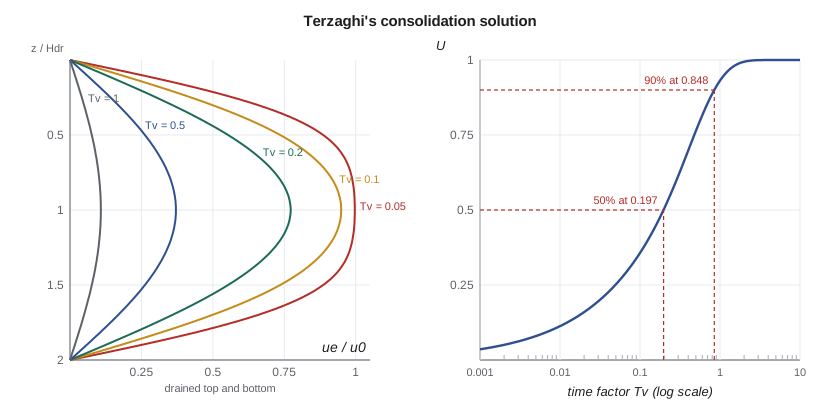
The isochrones show how consolidation proceeds: the clay near the drainage boundaries drains first, while the center of the layer stays at nearly the full excess pressure for a long time. The time to reach a given degree of consolidation is proportional to the square of the drainage path. Halving the drainage path cuts the time by four; this is the principle behind vertical drains.

Measuring cv

The coefficient of consolidation is found from the time-settlement record of each increment of the oedometer test. Two curve-fitting methods are standard. In Taylor's square-root-of-time method, the dial reading is plotted against \(\sqrt t\); the early part of the curve is a straight line, and a second line with abscissas 1.15 times as large cuts the curve at 90 % consolidation, giving \(t_{90}\). Then

In Casagrande's logarithm-of-time method, the end of primary consolidation is found as the intersection of the two straight parts of the curve of dial reading against \(\log t\), the start is found from the parabolic early part, and \(t_{50}\) gives \(c_v = 0.197H_{dr}^2/t_{50}\). The two methods usually agree within a factor of about 1.5. For the laboratory specimen, which drains at both faces, \(H_{dr}\) is half its thickness during the increment.

Drainage at the site

At the garage, the 23 ft clay layer lies between the sand above and the till below. The till is a silty sand with a permeability of perhaps \(10^{-5}\) cm/s, hundreds of times more permeable than the clay, so it acts as a drainage boundary. The drainage path is therefore half the layer, \(H_{dr} = 11.5\) ft.

These times assume a uniform initial excess pressure through the layer, which is true under a wide fill but not under a footing. Beneath the garage footing, most of the stress increase, and most of the settlement, is in the top meters of the clay, right next to the drainage boundary at the sand. That part consolidates much faster than the layer average. Sofia solves the consolidation equation numerically with the actual initial pressure profile from lesson 9, and weights each sublayer's progress by its share of the final settlement from lesson 10.

# Rate of consolidation of the site clay: cv, Terzaghi's solution, a numerical model and drains
from math import pi, exp, log, log10, sqrt

# 1. cv from Taylor's square-root-of-time fit (1 to 2 tsf increment, specimen 0.75 in. thick, drained both faces)
Hdr_lab, t90_lab = 0.375 / 12, 960.0       # ft, s
cv = 0.848 * Hdr_lab ** 2 / t90_lab        # ft2/s
cv_y = cv * 3.156e7                        # ft2/year
print(f"cv = {cv * 929.03:.2e} cm2/s = {cv_y:.1f} ft2/year")
mv = (1.033 - 0.957) / ((1 + 1.033) * 2000.0)  # 1/psf over the same increment
k = cv * mv * 62.4 * 30.48                 # cm/s
print(f"mv = {mv:.2e} 1/psf;  k = cv mv gamma_w = {k:.1e} cm/s")

# 2. Terzaghi's average degree of consolidation for a uniform initial excess pore pressure
def U(Tv, terms=50):
    return 1 - sum(2 / ((pi * (2 * m + 1) / 2) ** 2) * exp(-((pi * (2 * m + 1) / 2) ** 2) * Tv) for m in range(terms))
print("\n  Tv     U")
for Tv in (0.05, 0.1, 0.197, 0.3, 0.5, 0.848, 1.0):
    print(f"{Tv:5.3f}  {U(Tv):5.3f}")
Hdr = 11.5                                 # 23 ft of clay drained to the sand above and the till below
for Ux, Tv in ((50, 0.197), (90, 0.848)):
    print(f"t{Ux} for the clay layer = {Tv * Hdr ** 2 / cv_y:.1f} years")

# 3. Explicit finite differences with the real initial excess pressure under the footing
dz, H = 0.5, 23.0
n = int(H / dz) + 1
def dsig(z):                               # stress increase below the footing (lesson 9), z from the top of the clay
    pts = [(0, 2010.0), (4, 1224.0), (8, 863.0), (11.5, 700.0), (17, 557.0), (23, 460.0)]
    for (z1, s1), (z2, s2) in zip(pts, pts[1:]):
        if z1 <= z <= z2:
            return s1 + (s2 - s1) * (z - z1) / (z2 - z1)
u = [dsig(i * dz) for i in range(n)]; u[0] = u[-1] = 0.0   # drained top and bottom
u0 = [dsig(i * dz) for i in range(n)]
sub = [0.95, 0.52, 0.25, 0.13, 0.10, 0.09, 0.08, 0.07]     # final settlement of each sublayer (in.), lesson 10
th = H / len(sub)
dt = 0.4 * dz ** 2 / cv_y
t, report = 0.0, [0.25, 0.5, 1, 2, 4, 8]
print("\n years   U (uniform theory)   settlement (numerical)")
while report:
    t += dt
    u = [0.0] + [u[i] + cv_y * dt / dz ** 2 * (u[i + 1] - 2 * u[i] + u[i - 1]) for i in range(1, n - 1)] + [0.0]
    if t >= report[0]:
        s = 0.0
        for k in range(len(sub)):
            idx = [i for i in range(n) if k * th <= i * dz <= (k + 1) * th]
            Uk = 1 - sum(u[i] for i in idx) / sum(u0[i] for i in idx)
            s += sub[k] * Uk
        Tv = cv_y * report[0] / Hdr ** 2
        print(f"{report[0]:5.2f}       {U(Tv):5.2f}              {s:5.2f} in. of {sum(sub):.2f}")
        report.pop(0)

# 4. Prefabricated vertical drains for an alternative preload of the yard (Barron/Hansbo, no smear)
ch = 3 * cv_y                              # horizontal cv, higher in the varved clay
s_drain, dw = 5.0, 2.0 / 12                # triangular spacing and equivalent drain diameter (ft)
de = 1.05 * s_drain; nn = de / dw; F = log(nn) - 0.75
for Uh in (0.5, 0.9):
    Th = -log(1 - Uh) * F / 8
    print(f"Drains at {s_drain:.0f} ft: Uh = {Uh:.0%} after {Th * de ** 2 / ch * 12:.1f} months")

# 5. Secondary compression over 50 years after primary consolidation
t_p = 4.0
for name, Ca, Hs, ep in (("upper 10 ft, normally consolidated range", 0.008, 10.0, 0.96), ("lower 13 ft, overconsolidated", 0.003, 13.0, 1.00)):
    ss = Ca / (1 + ep) * Hs * log10(50 / t_p)
    print(f"Secondary settlement, {name}: {12 * ss:.2f} in.")

cv = 8.01e-04 cm2/s = 27.2 ft2/year
mv = 1.87e-05 1/psf;  k = cv mv gamma_w = 3.1e-08 cm/s

  Tv     U
0.050  0.252
0.100  0.357
0.197  0.500
0.300  0.613
0.500  0.764
0.848  0.900
1.000  0.931
t50 for the clay layer = 1.0 years
t90 for the clay layer = 4.1 years

 years   U (uniform theory)   settlement (numerical)
 0.25        0.26               1.01 in. of 2.19
 0.50        0.36               1.25 in. of 2.19
 1.00        0.51               1.51 in. of 2.19
 2.00        0.71               1.79 in. of 2.19
 4.00        0.89               2.05 in. of 2.19
 8.00        0.99               2.17 in. of 2.19
Drains at 5 ft: Uh = 50% after 0.9 months
Drains at 5 ft: Uh = 90% after 3.1 months
Secondary settlement, upper 10 ft, normally consolidated range: 0.54 in.
Secondary settlement, lower 13 ft, overconsolidated: 0.26 in.

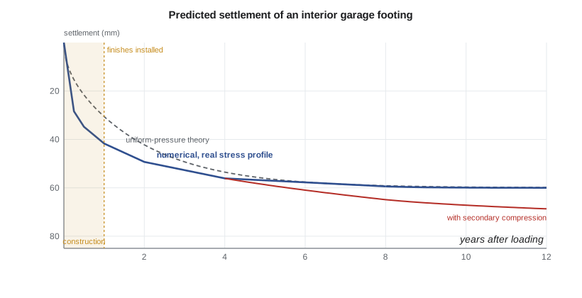
The numerical model shows almost half the settlement, 1.0 in., occurring within three months, 1.5 in. within a year and 2.05 in. within four years, compared with the uniform theory's 26 %, 51 % and 89 %. The garage will be under construction for about a year after the footings are poured, so roughly two thirds of the consolidation will have happened before the floor slab and finishes are placed.

Field values of cv

Field consolidation is often faster than laboratory tests predict. Thin sand and silt layers, fissures and root holes shorten the drainage paths, and the small laboratory specimen misses them. In varved clays the horizontal coefficient \(c_h\) can be several times \(c_v\). Back-analysis of settlement records from structures on the same deposit, or from piezometers and settlement plates during construction, gives the best values. For the yard fill, Dr. Kowalczyk specifies settlement plates and piezometers, so the predictions can be checked and updated with the observational method.

Preloading and vertical drains

When settlement would take too long, the site can be preloaded: a temporary fill is placed over the area, held until the clay has consolidated under it, and removed before construction. If the preload is heavier than the permanent load, the clay becomes overconsolidated with respect to the final load and later settles very little. A surcharge is the extra height above the permanent fill. Preloading is cheap but slow, so it is usually combined with vertical drains.

Prefabricated vertical drains (PVDs), plastic strips about 100 mm wide wrapped in a geotextile filter, are pushed into the clay on a grid at spacings of 1 to 3 m. Water flows horizontally to the nearest drain and up to a sand blanket at the surface. The drainage path becomes half the drain spacing instead of half the layer thickness, and the horizontal permeability, higher in layered clays, controls the flow. Barron's theory, simplified by Hansbo, gives the degree of consolidation by radial flow as

where \(d_e\) is the diameter of the soil cylinder drained by each drain, 1.05 times the spacing for a triangular pattern and 1.13 times for a square one, and \(n = d_e/d_w\) is its ratio to the equivalent drain diameter. Smear from installation and the drain's own flow resistance slow the process and are added to \(F(n)\) in design.

Secondary compression

After the excess pore pressure has dissipated, clays continue to compress slowly under constant effective stress as the particles creep and rearrange. This secondary compression is linear with the logarithm of time and is described by the secondary compression index

where \(e_p\) is the void ratio at the end of primary consolidation and \(t_1\) is that time. Mesri found that \(C_\alpha/C_c\) is roughly constant for a given soil, about 0.04 for inorganic clays and silts, 0.05 to 0.06 for organic clays and higher for peat. In the overconsolidated range, \(C_\alpha\) is much smaller, which is one reason preloading with a surcharge works so well: it pushes the clay into the overconsolidated range for the final load.

For the site clay, \(C_\alpha \approx 0.025C_c = 0.008\) in the upper part where the footing load exceeds \(\sigma'_p\), and about 0.003 below. Between the end of primary consolidation at about 4 years and a design life of 50 years, the script estimates about 0.8 in. of secondary settlement, more than a third as much as the primary. Most of it occurs slowly enough for the structure to accommodate.

Limits of the theory

Terzaghi's theory assumes constant \(c_v\), small strains and one-dimensional flow, and it separates primary from secondary compression. Real clays violate all of these to some degree: \(c_v\) changes as the clay stiffens, large settlements of soft clays change the drainage path, flow under a footing is three-dimensional, which speeds consolidation, and creep happens during primary consolidation as well as after it. Finite element programs with elastoplastic and creep models handle these effects for major projects. For most structures, the classical theory with good parameters and field monitoring gives answers well within the uncertainty of the soil properties.

Practical points

• Identify every drainage boundary, including thin sand and silt layers within the clay.
• Use the actual distribution of excess pore pressure when most of the load is near one boundary.
• Expect field consolidation to be faster than laboratory predictions in layered or fissured clays.
• Monitor settlements and pore pressures under fills; update predictions as data come in.
• Include secondary compression for organic soils and for long design lives.