Property relations and residual properties

Equations of state give pressure, volume and temperature. Energy balances need enthalpy, and second-law analyzes need entropy. The bridge between them is a set of exact mathematical relations among thermodynamic properties, derived once from the first and second laws and valid for every substance. With them, Theo can take the Peng-Robinson equation he set up for carbon dioxide in Lesson 4 and calculate how much the enthalpy of the gas changes between the compressor suction and the 20 bar intercooler outlet, how much it cools when throttled, and what heat capacity it really has at high pressure. This lesson develops those relations and the practical device that makes them easy to use: residual properties.

The fundamental property relations

For a closed system undergoing a reversible process, the first law gives \(dU = dQ_{rev} + dW_{rev}\), with \(dQ_{rev} = T\,dS\) from the second law and \(dW_{rev} = -P\,dV\). The result, \(dU = T\,dS - P\,dV\), contains only properties, so it holds for any process between equilibrium states, reversible or not. Three more relations follow by defining the enthalpy \(H = U + PV\), the Helmholtz energy \(A = U - TS\) and the Gibbs energy \(G = H - TS\). Each relation shows the natural variables of its property.

The Gibbs energy is especially important in chemical engineering because its natural variables, temperature and pressure, are the ones engineers control. At constant temperature and pressure, a system at equilibrium has the minimum possible Gibbs energy, which is the basis for phase and reaction equilibrium in Thermodynamics II.

Maxwell relations

Each fundamental relation is an exact differential, so its mixed second derivatives are equal. That gives four Maxwell relations. Two are used constantly, because they convert entropy derivatives, which cannot be measured directly, into PVT derivatives, which an equation of state supplies.

Enthalpy and entropy as functions of T and P

Engineers usually know temperature and pressure, so the most useful results express \(dH\) and \(dS\) in terms of \(dT\) and \(dP\). Starting from \(dH = T\,dS + V\,dP\), writing \(dS\) in terms of \(dT\) and \(dP\), and using the first Maxwell relation gives two general equations. The temperature terms involve the heat capacity, the pressure terms only volumetric data.

For an ideal gas, \(V - T(\partial V/\partial T)_P = 0\) and \((\partial V/\partial T)_P = R/P\), which recovers the results of Lessons 3 and 7: enthalpy depends on temperature only, and entropy has the \(-R\ln(P_2/P_1)\) term. For a liquid, with \(\beta = (1/V)(\partial V/\partial T)_P\), the pressure term in \(dH\) becomes \(V(1 - \beta T)\,dP\), small but sometimes worth including for high-pressure pumps.

The same derivation applied to a two-phase system gives the Clapeyron equation from Lesson 6. Along the vapor pressure curve, the Gibbs energies of the coexisting liquid and vapor stay equal, so \(dG^l = dG^v\), which with \(dG = -S\,dT + V\,dP\) and \(\Delta S^{lv} = \Delta H^{lv}/T\) gives \(dP^{sat}/dT = \Delta H^{lv}/(T\,\Delta V^{lv})\) exactly.

Residual properties

Integrating the general equations directly is awkward, because heat capacities of real fluids depend on pressure. Residual properties avoid that problem. The residual value of any property is the difference between its actual value and the value the same substance would have as an ideal gas at the same temperature and pressure. Because ideal gas properties are easy to compute and residual properties come straight from an equation of state, the actual property is simply the sum of the two.

Residual properties are found by integrating the general equations at constant temperature from zero pressure, where every fluid is ideal and residuals vanish, up to the actual pressure. In terms of the compressibility factor they become integrals of PVT data alone. The second equation shows how the residual Gibbs energy leads to the fugacity coefficient, the property Thermodynamics II uses for phase equilibrium.

With the truncated virial equation and the Pitzer correlation, the integrals give simple closed forms. With a cubic equation of state, they give closed forms in \(Z\), \(A\) and \(B\). The first equation below is the virial result for the residual enthalpy; the second pair gives the Peng-Robinson residual enthalpy and entropy, using \(a\) and its temperature derivative from Lesson 4.

Calculating a real-gas enthalpy change

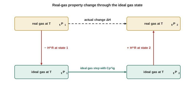
To find the change in enthalpy between two real states, follow a three-step path through the ideal gas state. First, remove the residual at the initial state, turning the real gas into an ideal gas at the same temperature and pressure. Second, change the ideal gas from the initial to the final temperature and pressure using ideal gas heat capacities. Third, add the residual at the final state. Entropy works the same way, with the ideal gas step including the pressure term.

Residual properties are what process simulators compute behind every enthalpy and entropy they report. When you choose a property method in a simulator, such as Peng-Robinson or Lee-Kesler, you are choosing the equation of state that supplies the residuals; the ideal gas heat capacities come from a separate database. Errors in either part show up in energy balances, so a quick hand check of one residual, with the virial correlation at moderate pressure, is a good habit when a simulation result looks surprising.

Real-gas heat capacity and the Joule-Thomson effect

Residual properties also explain two effects that ideal gas models miss. First, the heat capacity of a real gas at high pressure is larger than the ideal gas value, because part of the energy added goes into pulling molecules apart against their attractions. For carbon dioxide at 20 bar and 35 °C, the Peng-Robinson equation gives \(C_P\) about 43 J/(mol·K), against about 38 J/(mol·K) for the ideal gas. Near the critical point the difference becomes very large.

Second, a real gas changes temperature when it flows through a valve, a throttling process at constant enthalpy. The rate of change of temperature with pressure at constant enthalpy is the Joule-Thomson coefficient. From the general equation for \(dH\), setting \(dH = 0\) gives it in terms of PVT data and the heat capacity. For an ideal gas it is zero. For most real gases at ordinary temperatures it is positive, so they cool when throttled; hydrogen and helium at room temperature are exceptions.

# Residual properties of carbon dioxide from the Peng-Robinson equation and the Pitzer virial correlation
import math
R = 8.314
def pr_state(T, P, Tc, Pc, w, phase="vap"):
    """Peng-Robinson: returns Z, residual enthalpy H^R (J/mol), residual entropy S^R (J/mol K), ln(fugacity coefficient)."""
    k = 0.37464 + 1.54226 * w - 0.26992 * w ** 2
    sa = 1 + k * (1 - math.sqrt(T / Tc))
    ac = 0.45724 * R ** 2 * Tc ** 2 / Pc
    a, b = ac * sa ** 2, 0.07780 * R * Tc / Pc
    dadT = -ac * k * sa / math.sqrt(T * Tc)
    A, B = a * P / (R * T) ** 2, b * P / (R * T)
    c2, c1, c0 = -(1 - B), A - 3 * B ** 2 - 2 * B, -(A * B - B ** 2 - B ** 3)
    p = c1 - c2 ** 2 / 3; q = 2 * c2 ** 3 / 27 - c2 * c1 / 3 + c0
    disc = (q / 2) ** 2 + (p / 3) ** 3
    if disc > 0:
        u, v = -q / 2 + math.sqrt(disc), -q / 2 - math.sqrt(disc)
        roots = [math.copysign(abs(u) ** (1 / 3), u) + math.copysign(abs(v) ** (1 / 3), v) - c2 / 3]
    else:
        r = math.sqrt(-(p / 3) ** 3); phi = math.acos(max(-1.0, min(1.0, -q / (2 * r)))); m = 2 * math.sqrt(-p / 3)
        roots = [m * math.cos((phi + 2 * math.pi * j) / 3) - c2 / 3 for j in range(3)]
    roots = sorted(z for z in roots if z > B)
    Z = roots[-1] if phase == "vap" else roots[0]
    L = math.log((Z + (1 + math.sqrt(2)) * B) / (Z + (1 - math.sqrt(2)) * B))
    HR = R * T * (Z - 1) + (T * dadT - a) / (2 * math.sqrt(2) * b) * L
    SR = R * math.log(Z - B) + dadT / (2 * math.sqrt(2) * b) * L
    lnphi = Z - 1 - math.log(Z - B) - A / (2 * math.sqrt(2) * B) * L
    return Z, HR, SR, lnphi

Tc, Pc, w = 304.2, 73.8e5, 0.224                    # carbon dioxide (approximate)
A_, B_, D_ = 5.457, 1.045e-3, -1.157e5              # ideal gas Cp/R = A + B T + D/T^2

def h_ig(T, T0=298.15):  return R * (A_ * (T - T0) + B_ / 2 * (T ** 2 - T0 ** 2) - D_ * (1 / T - 1 / T0))
def s_ig(T, P, T0=298.15, P0=1e5):
    return R * (A_ * math.log(T / T0) + B_ * (T - T0) - D_ / 2 * (1 / T ** 2 - 1 / T0 ** 2) - math.log(P / P0))

def virial_residuals(T, P):
    Tr, Pr = T / Tc, P / Pc
    B0, B1 = 0.083 - 0.422 / Tr ** 1.6, 0.139 - 0.172 / Tr ** 4.2
    dB0, dB1 = 0.675 / Tr ** 2.6, 0.722 / Tr ** 5.2
    HR = R * T * Pr * (B0 - Tr * dB0 + w * (B1 - Tr * dB1))
    SR = -R * Pr * (dB0 + w * dB1)
    return HR, SR

print("State          Z(PR)   H^R PR  H^R virial (J/mol)   S^R PR  S^R virial (J/mol K)")
for label, T, P in (("1.05 bar, 30 C", 303.15, 1.05e5), ("20 bar, 35 C", 308.15, 20e5), ("50 bar, 35 C", 308.15, 50e5)):
    Z, HR, SR, _ = pr_state(T, P, Tc, Pc, w)
    hv, sv = virial_residuals(T, P)
    print(f"{label:14s} {Z:6.3f} {HR:8.0f} {hv:10.0f} {SR:14.2f} {sv:10.2f}")

# Enthalpy and entropy change from suction to 20 bar and 35 C, real gas versus ideal gas
T1, P1, T2, P2 = 303.15, 1.05e5, 308.15, 20e5
_, HR1, SR1, _ = pr_state(T1, P1, Tc, Pc, w)
_, HR2, SR2, _ = pr_state(T2, P2, Tc, Pc, w)
dH_ig, dS_ig = h_ig(T2) - h_ig(T1), s_ig(T2, P2) - s_ig(T1, P1)
dH, dS = dH_ig + HR2 - HR1, dS_ig + SR2 - SR1
print(f"Suction to 20 bar, 35 C: dH ideal {dH_ig:6.0f}, real {dH:6.0f} J/mol; dS ideal {dS_ig:6.2f}, real {dS:6.2f} J/(mol K)")

# Joule-Thomson coefficient at 20 bar and 35 C: mu = -(dH/dP)_T / Cp
def H(T, P): return h_ig(T) + pr_state(T, P, Tc, Pc, w)[1]
dP, dT = 1e3, 0.01
dHdP = (H(T2, P2 + dP) - H(T2, P2 - dP)) / (2 * dP)
Cp = (H(T2 + dT, P2) - H(T2 - dT, P2)) / (2 * dT)
print(f"Real-gas Cp at 20 bar, 35 C = {Cp:.1f} J/(mol K) (ideal gas {R * (A_ + B_ * T2 + D_ / T2 ** 2):.1f})")
print(f"Joule-Thomson coefficient = {-dHdP / Cp * 1e5:.2f} K/bar")

State          Z(PR)   H^R PR  H^R virial (J/mol)   S^R PR  S^R virial (J/mol K)
1.05 bar, 30 C  0.995      -42        -43          -0.09      -0.10
20 bar, 35 C    0.896     -840       -799          -1.88      -1.81
50 bar, 35 C    0.710    -2473      -1996          -5.82      -4.53
Suction to 20 bar, 35 C: dH ideal    189, real   -609 J/mol; dS ideal -23.88, real -25.67 J/(mol K)
Real-gas Cp at 20 bar, 35 C = 43.2 J/(mol K) (ideal gas 37.9)
Joule-Thomson coefficient = 1.05 K/bar

The program shows the virial and Peng-Robinson residuals agreeing closely at 1 bar and within about 5 percent at 20 bar, then diverging at 50 bar, where the virial correlation is outside its range. The Joule-Thomson coefficient of carbon dioxide at 20 bar and 35 °C comes out at about 1.05 K/bar, so throttling the gas by 10 bar would cool it by about 10 K. Lesson 10 uses this effect, and Lesson 12 builds a liquefier around it.